The difference between lead buyers who build sustainable businesses and those who burn through capital chasing unprofitable leads comes down to one metric they either master or ignore: Customer Lifetime Value. This guide provides the complete framework for calculating, applying, and optimizing LTV to transform your lead buying operation.
Why Customer Lifetime Value Determines Lead Buying Success
Every lead purchase is a bet. You pay $50, $100, or $500 upfront, gambling that the consumer on the other end will become a customer worth far more than your acquisition investment. The leads that lose this bet destroy your margins. The leads that win it build your business.
Customer Lifetime Value (LTV) is the framework that turns this gamble into a calculated investment. LTV represents the total revenue a customer generates over their entire relationship with your business, minus the costs to serve them. When you know your LTV with precision, you know exactly what you can afford to pay for leads while remaining profitable.
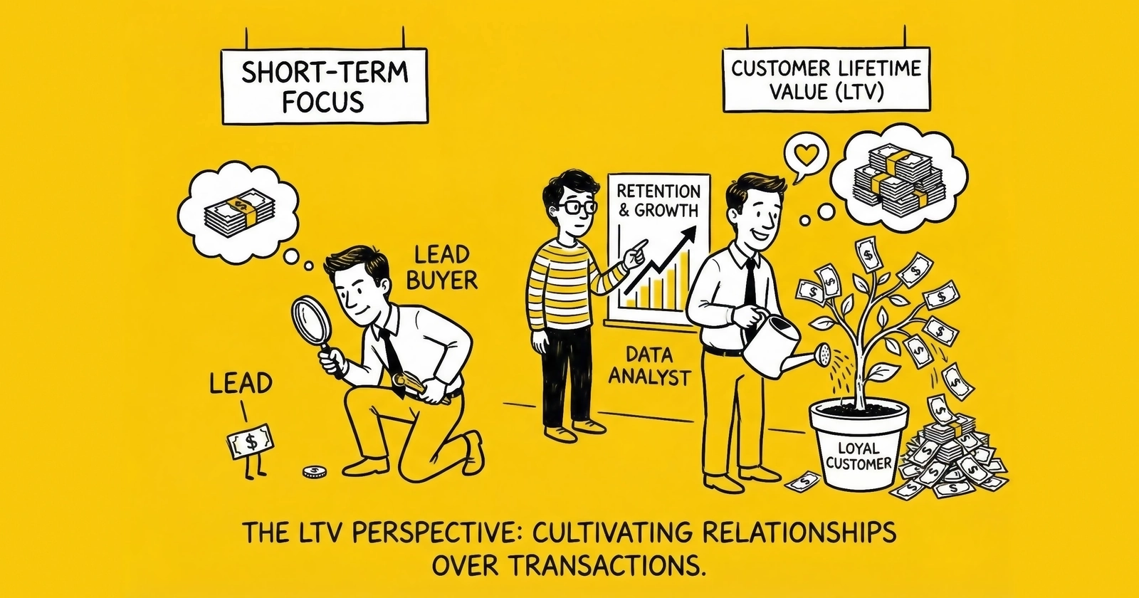
Most lead buyers get this wrong. They focus on cost per lead (CPL) as if cheaper leads automatically mean better returns. They celebrate when they negotiate a $5 discount on lead prices while ignoring that their customer retention dropped 10% – destroying far more value than they saved. They lack the unit economics foundation to make intelligent acquisition decisions.
Those who build sustainable lead-buying operations take a different approach. They calculate LTV by vertical, by lead source, by customer segment. They understand that a $100 lead converting to a customer worth $3,000 dramatically outperforms a $30 lead converting to a customer worth $500. They make acquisition decisions based on value creation, not cost minimization.
This guide provides everything you need to calculate LTV for your lead buying operation, apply that knowledge to acquisition decisions, and build the analytical infrastructure that separates professional operators from those running on intuition.
The Fundamentals of Customer Lifetime Value
What LTV Actually Measures
Customer Lifetime Value quantifies the total economic value a customer provides over their complete relationship with your business. This includes every transaction, every renewal, every referral, and every upsell – offset by the costs required to maintain that relationship.
The concept seems simple. The execution is anything but.
For a mortgage lender, LTV might include the initial loan origination fee, potential refinance transactions, cross-sold home equity lines, and referrals to the agent network – all extending over 7-10 years of homeownership. For an insurance agent, LTV includes first-year commissions, renewal commissions across multi-year policy retention, cross-sold additional lines (auto to home to umbrella), and the referral value of satisfied customers recommending family and friends.
The businesses that calculate LTV accurately understand their customers generate value across multiple dimensions and timeframes. Those that don’t consistently undervalue their acquisition capacity and leave growth on the table.
The Core LTV Formula
The basic LTV calculation follows this structure:
LTV = (Average Revenue per Customer) x (Gross Margin %) x (Average Customer Lifespan)
For a more sophisticated calculation that accounts for the time value of money:
LTV = (Average Monthly Revenue x Gross Margin %) x (1 / Monthly Churn Rate)
This formula recognizes that a dollar today is worth more than a dollar three years from now, and that retention rates directly determine how long customers generate value.
Consider an auto insurance agency with average annual premium of $1,400 and commission rate of 12%, yielding annual revenue per customer of $168. With average customer retention of 4.2 years and gross margin on servicing of 85%, the calculation follows:
LTV = $168 x 4.2 years x 0.85 = $599.76
That $600 LTV determines how much this agency can sustainably pay to acquire each customer. Understanding this number with precision – rather than guessing – is the foundation of profitable lead buying.
Why Most LTV Calculations Are Wrong
The formula above is deceptively simple. The inputs are where most practitioners fail.
Revenue underestimation plagues the majority of LTV calculations. Many practitioners only include primary product revenue, ignoring cross-sell, upsell, and referral value entirely. An auto insurance customer who adds a home policy and refers two neighbors generates 3-4x the value of the same customer measured only on auto premiums – yet most calculations miss this entirely.
Retention rate errors compound the problem. Using industry averages rather than your actual retention rates produces meaningless LTV figures. An agency with 90% annual retention generates dramatically different LTV than one with 75% retention – even with identical initial customer value. The difference in customer lifespan alone changes LTV by nearly 3x.
Margin confusion leads operators to inflate LTV and overpay for leads. Your LTV calculation should use gross margin (revenue minus cost of goods sold), not net margin (which includes overhead allocation). Confusing the two can make unprofitable acquisition appear sustainable.
Cohort blindness – treating all customers as identical – ignores that leads from different sources convert to customers with vastly different lifetime values. Your direct mail customers might retain 4.5 years while your shared lead customers retain only 2.8 years. Averaging these together obscures actionable intelligence.
Time horizon mismatch creates the most dangerous errors. Using 10-year LTV to justify acquisition costs for a business that might not exist in 10 years makes capital allocation decisions that can sink the entire operation.
Those who calculate LTV correctly start with verified data, segment by source and customer type, and update calculations quarterly as new information becomes available.
LTV Calculation Methods: Choosing Your Approach
Different businesses require different LTV calculation approaches based on data availability, business maturity, and customer relationship patterns.
Method 1: Historical LTV (Actual Data)
The most accurate LTV calculation uses actual customer data from your existing customer base. The formula is straightforward: divide total revenue from a customer cohort by the number of customers in that cohort.
Implementation requires four steps. First, select a customer cohort – for example, all customers acquired in Q1 2022. Second, track all revenue from that cohort through the present. Third, divide total revenue by the number of customers acquired. Finally, if the cohort is still active, project remaining value based on retention trends.
Consider a practical example. An operation acquired 200 customers in Q1 2022, generating total revenue of $340,000 through Q4 2024. With 142 customers still active (71% retained after 2.75 years) and projected remaining value of $85,000 based on the retention curve, actual LTV equals ($340,000 + $85,000) / 200 = $2,125.
The advantage of historical LTV is accuracy – it reflects your actual business performance rather than assumptions. The limitation is patience: this method requires 2-3 years of data minimum and cannot predict LTV for new customer segments or lead sources where you lack historical performance.
Method 2: Predictive LTV (Formula-Based)
When historical data is insufficient, formula-based predictions provide useful estimates. The basic formula is LTV = ARPC x AGM x (1 / Churn Rate), where ARPC represents Average Revenue Per Customer per period, AGM is Average Gross Margin percentage, and Churn Rate is the percentage of customers lost per period (matching the ARPC period).
Consider a mortgage broker building an LTV estimate. With average commission per loan of $4,500, average loans per customer lifetime of 1.3 (including refinances), and referral value of $750 (0.5 referrals x $1,500 value each), total ARPC reaches $6,600. Applying the formula with 90% gross margin yields LTV = $6,600 x 0.90 = $5,940.
This method offers immediate calculation without waiting years for cohort data, and allows scenario modeling to test different assumptions. The limitation is sensitivity – small changes in inputs produce large swings in output, making validation against actual data essential once available.
Method 3: Cohort-Based LTV
The most sophisticated approach tracks customer cohorts over time, revealing how different acquisition sources, time periods, and customer segments generate different lifetime values.
Implementation follows a systematic process. Define cohorts by acquisition month, source, or segment, then track each cohort’s monthly revenue and churn independently. Calculate cumulative LTV at each time interval and build LTV curves showing value accumulation over time. This creates a dynamic view of customer value that simple averages cannot provide.
The following cohort analysis illustrates the power of this approach:
| Months Since Acquisition | Cumulative LTV - Direct Mail | Cumulative LTV - Shared Leads | Cumulative LTV - Exclusive Leads |
|---|---|---|---|
| 3 | $245 | $180 | $320 |
| 6 | $465 | $310 | $580 |
| 12 | $820 | $485 | $1,050 |
| 24 | $1,450 | $720 | $1,890 |
| 36 | $1,980 | $890 | $2,520 |
This analysis reveals that exclusive leads generate 2.8x the lifetime value of shared leads – justifying substantially higher acquisition costs despite similar initial conversion rates.
The advantages of cohort-based analysis are substantial: it reveals source-specific and segment-specific LTV differences invisible to simpler methods, enabling precise acquisition targeting. The limitations are real, however. This approach requires sophisticated data infrastructure and grows complex to maintain across multiple dimensions. Most operations need dedicated analytics resources to sustain cohort tracking at scale.
Method 4: Probabilistic LTV Models
For mature operations with robust data, machine learning models predict individual customer LTV based on observable characteristics at acquisition.
These models draw on multiple predictive features: lead source and quality indicators, customer demographics and firmographics, initial purchase behavior, early engagement patterns, credit characteristics (where applicable), and geographic market factors. The output includes predicted LTV for each new customer, confidence intervals around those predictions, and feature importance rankings that reveal which characteristics matter most.
The advantages are powerful – probabilistic models enable real-time lead valuation and dynamic bid optimization while capturing complex relationships invisible to simple formulas. The limitations are equally significant: this approach requires substantial data science capability, carries high implementation cost, and demands ongoing monitoring for model drift as market conditions evolve.
LTV Benchmarks by Vertical
Understanding industry benchmarks provides context for your own LTV calculations and helps identify improvement opportunities.
Insurance Verticals
| Sub-Vertical | Customer LTV Range | Primary Value Drivers | Typical Retention |
|---|---|---|---|
| Auto Insurance | $1,500-$3,000 | 3-5 year retention, multi-policy bundling | 75-85% annual |
| Home Insurance | $2,000-$4,000 | Longer retention, bundling with auto | 85-90% annual |
| Life Insurance (Term) | $2,500-$5,000 | 10-20 year terms, conversion to permanent | Varies by term |
| Life Insurance (Whole) | $5,000-$15,000 | Lifetime relationship, accumulated value | 90%+ annual |
| Medicare Advantage | $1,200-$2,000 | Renewal commissions, product stability | 80-88% annual |
| Medicare Supplement | $1,800-$3,500 | Long retention, minimal churn | 90%+ annual |
| Health Insurance (ACA) | $800-$1,500 | Annual enrollment required, subsidy dependency | 65-75% annual |
| Commercial Insurance | $3,000-$15,000 | Multi-policy, longer relationships | 85-92% annual |
Key insight: Bundled insurance customers (auto + home) generate 2.5-3.5x the LTV of single-policy customers due to substantially higher retention rates (85-90% vs. 75-80%) and combined premium value.
Financial Services Verticals
| Sub-Vertical | Customer LTV Range | Primary Value Drivers | Typical Retention |
|---|---|---|---|
| Mortgage (Purchase) | $3,500-$8,000 | Loan origination, refinance potential, referrals | Transaction-based |
| Mortgage (Refinance) | $2,500-$5,500 | Lower acquisition intent, rate-driven | Transaction-based |
| Personal Loans | $800-$2,500 | Repeat borrowing, credit line increases | 25-40% reborrow |
| Debt Consolidation | $1,500-$4,000 | Larger loan amounts, lower repeat | 15-25% reborrow |
| Credit Cards | $1,000-$3,000 | Interest income, fee revenue, long tenure | 85-95% annual |
| Auto Loans | $1,200-$2,500 | 4-6 year terms, refinance opportunity | Term-based |
| Student Loans | $2,000-$5,000 | Long repayment, refinance potential | Term-based |
Key insight: Mortgage LTV extends beyond the initial transaction. Customers who purchase often refinance 2-4 times over their homeownership, and satisfied customers refer 1.5-2.5 additional borrowers over their relationship.
Home Services Verticals
| Sub-Vertical | Customer LTV Range | Primary Value Drivers | Typical Retention |
|---|---|---|---|
| Solar Installation | $5,000-$15,000 | Large initial transaction, referral value | Transaction-based |
| HVAC | $1,500-$4,000 | System replacement + ongoing maintenance | Service relationship |
| Roofing | $2,000-$6,000 | Large project, referral and repeat | 10-15 year cycle |
| Pest Control | $2,000-$5,000 | Recurring monthly service | 70-80% annual |
| Pool Service | $8,000-$15,000 | Weekly maintenance over 5-7 years | 75-85% annual |
| Landscaping | $4,500-$14,000 | Recurring maintenance, seasonal upsells | 70-80% annual |
| Home Security | $1,500-$3,500 | Monthly monitoring over 3-5 years | 80-85% annual |
Key insight: Recurring service businesses (pest control, pool, landscaping) generate substantially higher LTV per customer than transaction-based businesses, justifying premium lead acquisition costs.
Legal Verticals
| Sub-Vertical | Customer LTV Range | Primary Value Drivers | Typical Retention |
|---|---|---|---|
| Personal Injury | $8,000-$25,000+ | Case settlement percentages | Case-based |
| Mass Tort | $5,000-$15,000 | Volume, case qualification rates | Case-based |
| Workers Compensation | $4,000-$12,000 | State fee structures, case complexity | Case-based |
| Family Law | $3,000-$10,000 | Hourly billing, case duration | Case-based |
| Estate Planning | $1,500-$5,000 | Initial planning + ongoing updates | Relationship-based |
| Criminal Defense | $5,000-$15,000 | Case type, urgency premium | Case-based |
Key insight: Legal LTV depends heavily on case qualification and retention through litigation. A lead that signs but fails to prosecute the case generates zero LTV regardless of initial acquisition cost.
The LTV:CAC Ratio: The Sustainability Test
Understanding LTV in isolation is insufficient. The relationship between lifetime value and customer acquisition cost (CAC) determines whether your lead buying operation is sustainable, scaling appropriately, or heading toward collapse.
Understanding the LTV:CAC Ratio
The LTV:CAC Ratio equals Customer Lifetime Value divided by Customer Acquisition Cost. This simple formula carries profound implications for acquisition strategy.
Customer Acquisition Cost (CAC) must include all costs to acquire a customer – not just lead purchase price. A complete CAC calculation includes lead purchase cost, cost of leads that did not convert (failed attempts), sales labor cost per acquired customer, technology and integration costs, compliance and verification costs, and management overhead allocation.
Consider a complete CAC example. With lead cost of $75, leads required per closed customer of 12 (8.3% conversion), total lead cost reaches $900 per customer. Add sales labor cost of $150 (3 hours at $50/hour) and technology/compliance allocation of $50, and total CAC equals $1,100. If LTV is $3,300, the LTV:CAC ratio equals $3,300 / $1,100 = 3:1.
Interpreting LTV:CAC Ratios
| LTV:CAC Ratio | Interpretation | Strategic Implication |
|---|---|---|
| Below 1:1 | Losing money on every customer | Immediate intervention required |
| 1:1 to 2:1 | Marginal or break-even economics | Unsustainable without improvement |
| 2:1 to 3:1 | Acceptable for high-volume, quick-payback businesses | Viable but limited margin |
| 3:1 to 5:1 | Healthy economics | Target range for most operations |
| 5:1 to 7:1 | Strong economics | Consider accelerating investment |
| Above 7:1 | Exceptional – or underinvesting in growth | Evaluate growth opportunities |
Target benchmarks vary by buyer type. Direct carriers and lenders typically require 3:1 to 4:1 LTV:CAC for sustainable acquisition given their longer payback tolerance. Agents and brokers work with 2.5:1 to 3.5:1 ratios due to faster payback requirements and tighter cash constraints. Call centers and aggregators need 4:1 to 5:1 ratios to cover their higher operational overhead and thinner margins per customer.
CAC Payback Period
LTV:CAC ratio tells you whether acquisition is profitable. CAC payback period tells you how long that profitability takes to materialize. The formula is straightforward: CAC Payback Period = CAC / (Monthly Revenue x Gross Margin).
Consider an example with CAC of $1,100, monthly revenue per customer of $125, and gross margin of 80%. Monthly gross profit equals $100, yielding CAC payback of $1,100 / $100 = 11 months.
Payback period benchmarks follow a clear hierarchy. Under 6 months represents excellent cash efficiency – you recover acquisition costs quickly and can reinvest rapidly. 6-12 months is healthy for most businesses, balancing growth speed with capital requirements. 12-18 months is acceptable for high-LTV relationships where the long-term value justifies the wait. 18-24 months requires strong retention and capital access to survive the extended investment period. Over 24 months is dangerous without external funding.
The capital implications deserve emphasis. Long payback periods require substantial working capital. A business acquiring 100 customers monthly at $1,100 CAC with 12-month payback needs $1.32 million in working capital just to fund acquisition – before any operational expenses. Many operations that appear profitable on an LTV basis fail because they underestimate the cash required to survive until that profitability materializes.
Common LTV:CAC Calculation Errors
Several calculation errors consistently undermine LTV:CAC analysis.
Ignoring lead waste is the most common mistake. Many buyers calculate CAC using only the cost of leads that converted, ignoring the majority that did not. If you buy 100 leads at $50 each and 8 convert, your lead cost per customer is $625, not $50. This error alone can cause a 10x understatement of true acquisition cost.
Excluding sales costs compounds the problem. Lead cost is only part of CAC. The sales labor, technology, and overhead required to work those leads often doubles or triples true acquisition cost. An operation that believes CAC is $50 when it is actually $200 will make disastrous acquisition decisions.
Using gross LTV against partial CAC creates false confidence. Comparing full LTV (including future value that takes years to materialize) against incomplete CAC that excludes most costs produces ratios that look healthy but reflect fantasy economics. Use consistent, complete definitions for both metrics.
Ignoring customer quality variation leads to averaged decisions that destroy value. Not all customers are equal. Leads from certain sources may convert but generate customers who churn faster, claim more service, or never cross-sell – reducing LTV even when conversion rates look acceptable. Source-level LTV analysis reveals these differences; averaged calculations hide them.
Cohort-Based LTV Analysis: The Professional Approach
Simple LTV averages hide more than they reveal. Professional lead buyers analyze LTV by cohort – grouping customers by acquisition source, time period, and characteristics – to understand which leads generate profitable customers and which destroy value.
Building Cohort Analysis Infrastructure
Effective cohort analysis requires tracking customers from acquisition through their entire lifecycle. The required data elements span the complete customer journey: original lead source and campaign, acquisition date, lead cost, conversion date, customer segment assignment, monthly revenue by customer, churn date (when applicable), all cross-sell and upsell transactions, and referral attribution. Missing any of these elements creates blind spots in your analysis.
The cohort dimensions you track determine what questions you can answer. Time-based cohorts (acquisition month or quarter) reveal seasonality and trend changes. Source-based cohorts (lead vendor, channel, or campaign) identify which acquisition investments generate the best customers. Quality-based cohorts (lead score tier, qualification level) validate whether your scoring actually predicts customer value. Segment-based cohorts (customer type, product category, geography) uncover which market segments deserve investment. Price-based cohorts (lead cost tier, bid level) test whether paying more for leads actually delivers proportionally better customers.
Interpreting Cohort Curves
LTV curves show how value accumulates over time for different customer groups. Reading these curves correctly reveals the health of your customer relationships.
Healthy cohort curves share common characteristics. They show steep initial value accumulation, indicating strong early monetization. The curve gradually flattens as natural retention decay occurs, but maintains a long tail where retained customers continue generating value. Visible bumps appear as cross-sell events add value beyond initial products.
Warning signals in cohort curves demand attention. Rapid early plateau indicates customers are not retained past the initial transaction – you may be attracting deal-seekers who extract value and leave. Steep mid-curve drops suggest quality or service problems driving churn after the honeymoon period. Flat tails reveal absence of cross-sell or repeat purchase behavior, limiting customer value to initial transactions. Erratic patterns often indicate data quality or tracking issues rather than true customer behavior – investigate before drawing conclusions.
Source-Level LTV Comparison
The most actionable cohort insight compares LTV across lead sources.
Example analysis:
| Lead Source | Lead CPL | Conversion Rate | CAC | 12-Month LTV | 36-Month LTV | LTV:CAC |
|---|---|---|---|---|---|---|
| Vendor A | $45 | 12% | $375 | $680 | $1,890 | 5.0:1 |
| Vendor B | $65 | 8% | $812 | $720 | $2,150 | 2.6:1 |
| Vendor C | $35 | 15% | $233 | $410 | $980 | 4.2:1 |
| Direct Mail | $28 | 6% | $467 | $890 | $2,680 | 5.7:1 |
| Exclusive Leads | $120 | 18% | $667 | $1,050 | $2,920 | 4.4:1 |
The insights from this analysis reshape acquisition strategy. Vendor A offers the best immediate economics with the highest 12-month LTV:CAC ratio. Direct Mail generates the highest long-term value despite lower conversion rates, rewarding patience. Vendor C’s cheap leads convert well but generate low-quality customers whose value plateaus quickly. Exclusive leads justify their premium pricing through superior customer quality and long-term retention. Vendor B underperforms across all timeframes – reduce allocation or eliminate entirely.
This analysis enables data-driven lead source allocation rather than intuition-based decisions. Without source-level LTV tracking, you cannot know which acquisition investments create value and which destroy it.
Segment-Level LTV Differences
Customer characteristics visible at acquisition often predict lifetime value. The following insurance example illustrates how LTV varies by customer profile:
| Customer Segment | Lead Cost Premium | Conversion Rate | Average LTV | Recommended Bid Premium |
|---|---|---|---|---|
| Homeowners, Age 35-55 | +25% | 14% | $2,850 | +30% |
| Renters, Age 25-34 | Baseline | 10% | $1,200 | Baseline |
| Renters, Under 25 | -15% | 8% | $680 | -25% |
| Multi-vehicle households | +20% | 12% | $2,400 | +35% |
| Clean driving record | +15% | 15% | $2,100 | +25% |
| Prior incidents | -10% | 7% | $1,100 | -20% |
The actionable implication is clear: bid more aggressively for leads matching high-LTV profiles, even if CPL appears expensive. A homeowner aged 35-55 generates $2,850 in lifetime value versus $680 for a young renter – paying 25% more for that lead still delivers dramatically better economics. Conversely, reduce bids for segments that historically generate low LTV, even if conversion rates seem acceptable. High conversion on low-value customers is not a victory.
Predictive LTV Models: From Calculation to Optimization
Mature lead buying operations move beyond historical LTV calculation toward predictive models that estimate individual customer value at the point of lead purchase.
Why Predictive LTV Matters
Historical LTV tells you what happened. Predictive LTV tells you what to expect – enabling real-time acquisition decisions.
The capabilities predictive LTV unlocks transform acquisition strategy. You can bid more for leads likely to become high-value customers, winning competitive auctions for the prospects who matter most. You can decline leads predicted to generate low or negative value, avoiding the trap of paying for customers who destroy margins. You can allocate sales resources to high-potential leads, ensuring your best people work the best opportunities. You can forecast revenue more accurately, building plans on data rather than hope. You can optimize marketing spend toward high-LTV segments, directing budget where it generates the greatest return.
Building a Predictive LTV Model
Building a predictive LTV model requires four systematic steps.
Step 1: Define the Target Variable
What exactly are you predicting? The options carry different implications. Total revenue over 12, 24, or 36 months provides a straightforward target but ignores cost-to-serve. Cumulative gross margin accounts for service costs but requires more complex tracking. Revenue net of expected service costs offers the most accurate value measure but demands sophisticated cost attribution. Probability of reaching a value threshold (such as “will this customer generate $2,000+ in margin?”) simplifies the prediction to classification but loses granularity.
Step 2: Identify Predictive Features
Determining which lead and customer characteristics predict lifetime value requires both domain knowledge and data exploration. Common predictive features include lead source and campaign, geographic market (state, metro area, zip density), lead qualification responses (intent, timeline, budget), credit indicators (where available), demographic characteristics, time of submission (day of week, time of day), device and session characteristics, and prior relationship indicators. Not all features matter equally – feature importance analysis reveals which characteristics actually drive value.
Step 3: Build and Validate the Model
Use historical data to train models predicting LTV from available features. Regression models work for continuous LTV prediction when you need precise dollar estimates. Classification models suit LTV tier assignment when grouping customers into value buckets is sufficient. Survival analysis focuses on retention-driven predictions, particularly valuable when churn timing dominates value calculation. Machine learning ensembles capture complex patterns invisible to simpler approaches but require more sophisticated implementation.
Step 4: Implement and Monitor
Deploy predictions into acquisition workflows where they can influence decisions. Real-time bid adjustment in ping-post systems enables value-based purchasing. Lead routing to appropriate sales resources ensures high-potential leads get premium attention. Dashboard integration provides performance monitoring visibility. Automated alerts for model drift catch degradation before it destroys value. Models require ongoing maintenance – market conditions change, and yesterday’s predictive features may lose power over time.
Practical Predictive LTV Implementation
Even without data science resources, you can implement basic predictive LTV using lead characteristics. A simple scoring approach captures most of the value of sophisticated models.
The process is straightforward. First, identify 5-7 lead characteristics that correlate with LTV based on your historical data. Second, assign point values to each characteristic based on historical performance – characteristics that predict high LTV get more points. Third, sum points for each lead to create a predicted LTV score. Finally, map scores to LTV tier estimates that guide bidding and routing decisions.
The following scoring matrix illustrates the approach:
| Characteristic | High Value (3 pts) | Medium Value (2 pts) | Low Value (1 pt) |
|---|---|---|---|
| Property Status | Homeowner | Renter 2+ years | Renter <2 years |
| Age Range | 35-55 | 25-34 or 56-65 | Under 25 or 65+ |
| Credit Tier | 720+ | 650-719 | Under 650 |
| Intent Signal | Quote today | Quote this week | Just browsing |
| Multi-product | 2+ products | 1 product + interest | Single product only |
Score interpretation follows a tiered structure. Leads scoring 13-15 points qualify as premium tier, warranting bids at 130% of baseline. Scores of 10-12 points represent standard tier with baseline bidding. Scores of 7-9 points fall into discount tier with bids at 70% of baseline. Leads scoring under 7 points should be declined or receive only minimal bids.
This approach captures 70-80% of the value of sophisticated ML models while requiring only spreadsheet-level implementation. The key is calibrating point values to your actual historical data rather than guessing – even simple models work well when grounded in real performance.
Applying LTV to Lead Buying Decisions
Understanding LTV transforms lead buying from a cost-minimization exercise into a value-creation strategy.
Maximum Sustainable Lead Price Calculation
Your LTV determines the ceiling for sustainable lead prices. The formula is Maximum CPL = (LTV x Target Conversion Rate) / Target LTV:CAC Ratio.
Consider an example with customer LTV of $2,400, target conversion rate of 8%, and target LTV:CAC ratio of 3:1. Target CAC equals $2,400 / 3 = $800.
If leads cost 60% of CAC and sales costs comprise the remaining 40%, Maximum CPL equals $800 x 0.60 = $480. But that assumes 100% conversion. Adjusting for 8% conversion: Maximum CPL = $480 x 0.08 = $38.40.
At this price, you acquire customers for $480 in lead costs ($38.40 / 8%), leaving $320 for sales costs and achieving your target 3:1 LTV:CAC ratio. Understanding this math prevents both overpaying for leads and leaving growth on the table by bidding too conservatively.
Bid Optimization Using LTV
In competitive lead markets, LTV-based bidding creates sustainable advantage.
Most buyers use static pricing – they bid $45 for all auto insurance leads, accept whatever quality comes at that price, and hope economics work out. This approach treats all leads as equally valuable, which they are not.
LTV-optimized bidding takes a fundamentally different approach. Segment leads by predicted LTV tier. Bid $65 for leads matching high-LTV profiles – homeowners, multi-vehicle households, clean records. Bid $35 for leads matching low-LTV profiles – young renters, prior incidents, single policies. Bid $0 for leads unlikely to generate positive value.
The outcome transforms acquisition economics. You win more high-value leads because competitors using static bids get outbid on the opportunities that matter. You avoid low-value leads while competitors overpay for them. You achieve superior overall LTV:CAC despite higher average CPL because the leads you win are worth proportionally more than the premium you pay.
Portfolio Allocation by LTV
LTV analysis should drive how you allocate lead buying budget across sources.
The allocation framework follows a logical sequence. Rank all lead sources by LTV:CAC ratio to understand relative performance. Calculate marginal return for additional spend on each source – this often differs from average return as sources have diminishing returns at scale. Allocate incremental budget to highest marginal return sources first. Set floor allocations to maintain source diversity and avoid over-concentration risk. Review and rebalance quarterly as source performance shifts.
Consider the following allocation example:
| Lead Source | Current Spend | LTV:CAC | Marginal Return | Reallocation |
|---|---|---|---|---|
| Source A | $50,000 | 4.2:1 | $3.20 per $1 | +$15,000 |
| Source B | $40,000 | 3.8:1 | $2.80 per $1 | +$10,000 |
| Source C | $35,000 | 2.9:1 | $1.90 per $1 | Hold |
| Source D | $30,000 | 2.1:1 | $1.10 per $1 | -$10,000 |
| Source E | $25,000 | 1.5:1 | $0.50 per $1 | -$15,000 |
This reallocation moves $25,000 from low-performing sources to high-performing sources, improving overall portfolio returns without changing total spend.
Retention Impact on Acquisition Decisions
LTV-aware buyers recognize that retention rates dramatically affect acquisition economics. The following sensitivity analysis illustrates the impact for a customer generating $150 monthly gross profit:
| Annual Retention | Customer Lifespan | LTV | Max Sustainable CAC (3:1) |
|---|---|---|---|
| 70% | 3.3 years | $5,940 | $1,980 |
| 80% | 5.0 years | $9,000 | $3,000 |
| 85% | 6.7 years | $12,060 | $4,020 |
| 90% | 10.0 years | $18,000 | $6,000 |
The insight here is profound: improving retention from 80% to 85% increases LTV by 34% – the equivalent of finding leads 34% cheaper. Investing in customer success often generates better returns than negotiating harder on lead prices. A retention-focused operation can afford to pay more for leads than a churn-heavy competitor, creating sustainable acquisition advantage.
Building LTV Tracking Infrastructure
Calculating LTV once provides a snapshot. Building infrastructure for ongoing LTV tracking provides strategic advantage.
Essential Data Requirements
Customer-level tracking forms the foundation. Each customer record must include a unique identifier linking lead to customer, original lead source with campaign and cost data, all revenue transactions with dates, product holdings and changes over time, service interactions and costs, churn events with reasons, and referral relationships. Missing any of these elements creates blind spots that undermine analysis accuracy.
Aggregation requirements enable the analysis itself. Monthly cohort summaries allow trend tracking. Source-level performance aggregation reveals which acquisition investments work. Segment-level performance splits uncover customer type differences. Time-series LTV curve data shows how value accumulates over customer lifespans.
Integration requirements connect the data sources. Lead management systems must link to CRM records so you can track leads through conversion. CRM must connect to billing and transaction systems to capture revenue. Transaction data flows to analytics warehouses for processing. Analytics warehouses feed reporting and BI layers for visibility. Gaps in this chain create gaps in your understanding.
LTV Dashboard Design
Effective LTV dashboards organize around four question categories.
Portfolio health questions establish the baseline. What is current average LTV across all customers? How does LTV trend over time – improving, declining, or stable? Which segments are improving or declining relative to the overall trend?
Acquisition optimization questions guide spending decisions. What is LTV:CAC by lead source? Which sources are over or underperforming relative to their cost? Where should we increase or decrease spend to improve portfolio returns?
Cohort performance questions catch problems early. How do recent cohorts compare to historical norms? Are there early warning signals in new cohort curves – faster churn, lower initial monetization, weaker cross-sell? Which cohorts are outperforming or underperforming expectations, and why?
Segment insights questions reveal growth opportunities. Which customer segments generate highest LTV? Are high-LTV segments growing or shrinking as a share of acquisition? What characteristics predict segment membership, enabling better targeting?
Recommended Analytics Stack
The appropriate analytics stack depends on operation scale.
For startups and small operations, spreadsheet-based cohort tracking provides sufficient capability. Manual monthly LTV calculation, simple source-level comparison, and quarterly review cadence keep investment proportional to lead spend while building analytical muscle.
For mid-size operations spending $1M-$10M annually on leads, the requirements escalate. Dedicated analytics databases (Postgres, BigQuery) provide the processing power needed. BI tool integration (Looker, Tableau, PowerBI) enables visualization and exploration. Automated daily data refresh keeps analysis current. Weekly LTV reporting maintains visibility. Source-level bid optimization becomes feasible with reliable data infrastructure.
For enterprise operations spending $10M+ annually on leads, sophisticated infrastructure becomes essential. Data warehouses with full customer data integration support complex analysis. Real-time LTV prediction models enable dynamic bidding. Automated bid management systems execute decisions at scale. Daily cohort monitoring catches changes quickly. Predictive churn integration anticipates retention problems. A/B testing infrastructure supports acquisition experiments that improve performance over time.
Common LTV Mistakes and How to Avoid Them
Five mistakes consistently undermine LTV analysis. Understanding each error, its real-world impact, and the solution enables professional-grade LTV practice.
Mistake 1: Ignoring Customer Quality Variation
The error is treating all customers as equally valuable when calculating LTV. The reality is that customers from different lead sources, with different profiles, generate dramatically different lifetime values – often varying 3-5x within the same business. A young renter from a shared lead generates fundamentally different value than a homeowner from a referral. The solution is to segment LTV calculation by lead source, customer profile, and acquisition characteristics, using segment-specific LTV for acquisition decisions rather than business-wide averages.
Mistake 2: Using LTV to Justify Unprofitable Acquisition
The error is using long-term LTV projections to justify acquisition economics that require 3-5 years to reach profitability. The reality is that cash is required today, not in 3 years. Businesses that over-invest in acquisition based on distant LTV projections often run out of capital before those projections materialize. The solution is to constrain acquisition to levels supportable by available capital, calculate CAC payback period alongside LTV:CAC ratio, and ensure payback occurs within 12-18 months for most businesses.
Mistake 3: Overweighting Referral Value
The error is inflating LTV with optimistic referral projections that rarely materialize. The reality is that referral value is real but difficult to track and highly variable. Most businesses overestimate referral rates and underestimate the time and investment required to generate referrals. The solution is to include referral value only when you have verified historical data, use conservative estimates (50% of tracked rates), and track referral attribution systematically.
Mistake 4: Confusing Revenue with Profit
The error is calculating LTV using revenue rather than gross margin, then comparing to CAC that only includes lead costs. The reality is that serving customers has costs. A customer generating $10,000 in revenue but requiring $7,000 in service costs only contributes $3,000 to LTV. The solution is to always use gross margin-adjusted LTV, include cost-to-serve in customer value calculations, and compare margin-based LTV to fully-loaded CAC.
Mistake 5: Static LTV Calculation
The error is calculating LTV once and using that number indefinitely. The reality is that market conditions, customer behavior, product mix, and competitive dynamics all change. LTV calculated in 2022 may not reflect 2025 customer economics. The solution is to recalculate LTV quarterly using recent cohorts, track LTV trends over time, and adjust acquisition strategy as LTV changes.
Frequently Asked Questions
What is Customer Lifetime Value (LTV) in lead generation and why does it matter?
Customer Lifetime Value represents the total revenue a customer generates over their complete relationship with your business, minus the costs to serve them. For lead buyers, LTV determines what you can sustainably pay for leads while remaining profitable. A business that knows customers generate $2,400 in lifetime value can confidently pay more for quality leads than a competitor guessing at customer value. LTV transforms lead buying from cost minimization to value creation, enabling strategic decisions about acquisition investment, source selection, and growth acceleration.
How do I calculate LTV for my lead buying operation?
The core LTV formula is: LTV = (Average Revenue per Customer) x (Gross Margin %) x (Average Customer Lifespan). For more precision, use: LTV = (Average Monthly Revenue x Gross Margin %) x (1 / Monthly Churn Rate). Start by calculating average revenue per customer over their relationship, apply your gross margin percentage to get profit contribution, then multiply by average customer lifespan. For example, an insurance agent with $1,400 average annual premium, 12% commission rate ($168/year), 85% gross margin, and 4.2 year average retention has LTV of $168 x 4.2 x 0.85 = $600.
What LTV:CAC ratio should lead buyers target for sustainable economics?
Most lead buying operations should target 3:1 to 5:1 LTV:CAC ratio. Below 2:1 indicates unsustainable acquisition economics requiring immediate intervention. Between 2:1 and 3:1 is marginally viable but leaves limited margin for error. 3:1 to 5:1 represents healthy economics with room for growth investment. 5:1 to 7:1 suggests strong economics – consider accelerating acquisition. Above 7:1 either indicates exceptional performance or potential underinvestment in growth. Direct carriers and lenders typically require 3:1 to 4:1, agents and brokers work with 2.5:1 to 3.5:1, and call centers require 4:1 to 5:1 due to higher operational overhead.
How do I calculate Customer Acquisition Cost (CAC) correctly?
CAC includes all costs required to acquire a customer, not just lead purchase price. Calculate: Lead cost per customer = (Lead CPL x Number of leads purchased) / Number of customers acquired. If you buy 100 leads at $50 and convert 8 customers, lead cost per customer is $625. Then add sales labor cost (time spent x hourly rate), technology and integration costs, compliance and verification costs, and management overhead allocation. A complete CAC calculation might show: Lead cost $625 + Sales labor $150 + Technology $35 + Overhead $40 = $850 total CAC. Using only lead cost dramatically understates true acquisition cost.
How does retention rate affect LTV calculation?
Retention rate is the most powerful lever affecting LTV. The formula 1/Churn Rate directly determines customer lifespan. With 80% annual retention (20% churn), average customer lifespan is 5 years. With 90% retention (10% churn), lifespan doubles to 10 years. This means a 10-point retention improvement (80% to 90%) doubles your LTV without changing anything else about customer value. For a customer generating $1,500 in annual gross margin, improving retention from 80% to 90% increases LTV from $7,500 to $15,000. Often, investing in customer retention generates higher returns than negotiating lower lead prices.
What is cohort-based LTV analysis and why should I use it?
Cohort-based LTV analysis tracks customer groups by acquisition source, time period, or characteristics to understand how different segments generate different lifetime value. Instead of calculating one average LTV for all customers, you calculate separate LTV for customers from each lead source, each acquisition month, and each customer segment. This analysis reveals that exclusive leads might generate 2.5x the LTV of shared leads, or that customers acquired in Q1 retain 15% longer than Q4 acquisitions. Cohort analysis enables precise acquisition targeting – spending more on sources and segments that generate high-LTV customers while reducing investment in sources that destroy value.
How can I predict LTV for leads before purchasing them?
Predictive LTV uses observable lead characteristics to estimate customer lifetime value before acquisition. Basic approaches assign point values to characteristics that correlate with LTV (homeownership, age range, credit tier, intent signals) and sum points to create predicted value scores. Sophisticated approaches use machine learning models trained on historical data to predict LTV from lead attributes. Even simple predictive models enable bid optimization – paying more for leads matching high-LTV profiles and less for leads predicted to generate low-value customers. This creates sustainable competitive advantage versus buyers using static bidding.
What are the biggest mistakes lead buyers make with LTV calculation?
The most common mistakes include: treating all customers as equally valuable (ignoring that source-specific LTV often varies 3-5x), using long-term LTV to justify acquisition that requires years to become profitable (ignoring cash flow reality), overweighting referral value with optimistic projections, confusing revenue with profit (calculating LTV on revenue rather than margin), and calculating LTV once and never updating it (ignoring that customer economics change over time). Professional operators segment LTV by source and customer type, constrain acquisition to capital availability, use conservative referral estimates, always use margin-adjusted calculations, and recalculate LTV quarterly.
How should LTV inform my lead bidding strategy?
LTV-informed bidding replaces static pricing with value-based acquisition. Calculate maximum sustainable CPL for each lead type: Maximum CPL = (Predicted LTV x Expected Conversion Rate) / Target LTV:CAC Ratio. For segments with higher predicted LTV, bid more aggressively. For segments with lower predicted LTV, reduce bids or decline. Example: If standard leads generate $2,000 LTV and premium-profile leads generate $3,500 LTV, you can afford to bid 75% more for premium leads while maintaining the same return. This approach wins more high-value leads (outbidding competitors using static bids) while avoiding overpayment for low-value leads.
What data infrastructure do I need for LTV tracking?
Essential requirements include: unique customer identifiers linking leads to customer records, lead source and cost data persisted with customer records, all revenue transactions with dates, churn events with timing and reasons, and integration between lead management, CRM, and billing systems. For small operations, spreadsheet-based monthly tracking works. For mid-size operations ($1M-$10M lead spend), implement dedicated analytics databases with BI tool integration and weekly reporting. For enterprise operations, build data warehouses with real-time LTV prediction, automated bid management, and daily cohort monitoring. The investment in data infrastructure pays returns through superior acquisition decisions.
How often should I recalculate LTV for my business?
Recalculate LTV quarterly using your most recent 12-24 months of cohort data. Market conditions, competitive dynamics, product mix, and customer behavior all change over time. LTV calculated in 2022 may significantly misrepresent 2025 customer economics. Quarterly recalculation enables: trend identification (is LTV improving or declining?), early warning detection (are recent cohorts underperforming?), acquisition adjustment (should we change bid levels based on updated LTV?), and strategic planning (how does LTV trajectory affect growth plans?). Between quarterly recalculations, monitor leading indicators like retention rates and revenue per customer that might signal LTV changes before full cohort analysis confirms them.
Key Takeaways
Customer Lifetime Value is the foundation of sustainable lead buying economics. Those who master LTV calculation and application build businesses that compound value over time. Those who ignore it find themselves in a perpetual race to the bottom on lead prices while wondering why profitability remains elusive.
Seven essential principles define professional LTV practice:
- LTV determines what you can afford to pay for leads. The formula LTV = (Average Revenue x Gross Margin) x (1/Churn Rate) quantifies customer value and sets your acquisition ceiling. Know this number with precision for your business.
- LTV:CAC ratio is the sustainability test. Target 3:1 to 5:1 for healthy economics. Below 2:1 requires immediate intervention. Above 7:1 suggests potential underinvestment in growth.
- Retention is the highest-leverage LTV factor. Improving retention from 80% to 90% doubles average customer lifespan and roughly doubles LTV. Often, investing in retention generates higher returns than negotiating lower lead prices.
- Cohort-based analysis reveals source-level truth. Not all leads generate equal customer value. Track LTV by lead source, acquisition time, and customer segment to identify which sources create value and which destroy it.
- Predictive LTV enables bid optimization. Use lead characteristics to predict customer value before acquisition. Bid more for leads matching high-LTV profiles; decline leads predicted to generate negative value.
- CAC calculation must be complete. Include lead costs for unconverted leads, sales labor, technology, compliance, and overhead. Using only lead purchase price understates true acquisition cost by 40-60%.
- LTV requires ongoing measurement. Recalculate quarterly using recent cohort data. Customer economics change; your LTV calculations must reflect current reality rather than historical assumptions.
The math is unforgiving but illuminating. When you know your LTV with precision, every lead buying decision becomes clearer. You stop obsessing over CPL and start optimizing for customer value creation. You allocate budget to sources that generate profitable customers rather than cheap leads. You build the analytical infrastructure that separates professional operations from those running on intuition and hope.
Calculate your LTV. Understand your cohorts. Apply that knowledge to acquisition decisions. Those who do this systematically build sustainable competitive advantage in lead buying. The ones who do not remain forever vulnerable to competitors who understand the numbers better.
Sources
- Harvard Business Review - The Value of Keeping the Right Customers - Research on customer retention economics and LTV drivers
- Bain & Company - The Value of Online Customer Loyalty - Industry research on customer loyalty impact on lifetime value
- SuperOffice - Customer Retention Statistics - Verifies retention rate benchmarks and LTV impact data
- Klipfolio KPI Examples - Reference for LTV:CAC ratio benchmarks and calculation methodologies
- HubSpot Marketing Statistics - Industry benchmark data on customer acquisition costs and conversion rates
- Forrester Research - Source for enterprise data-driven business performance benchmarks
Statistics and benchmarks current as of late 2025. Customer economics, retention rates, and LTV calculations vary significantly by vertical, geography, and business model. Validate these frameworks against your own data before making significant acquisition decisions.