A comprehensive guide to building statistical models that predict lead conversion, identify quality drivers, and optimize your lead generation operation for maximum ROI.
Most lead generation operators think they understand what makes a quality lead. They point to obvious factors: valid phone numbers, correct email addresses, consumers who actually requested contact. These validation checks matter, but they explain perhaps 20% of why some leads convert and others disappear into the void.
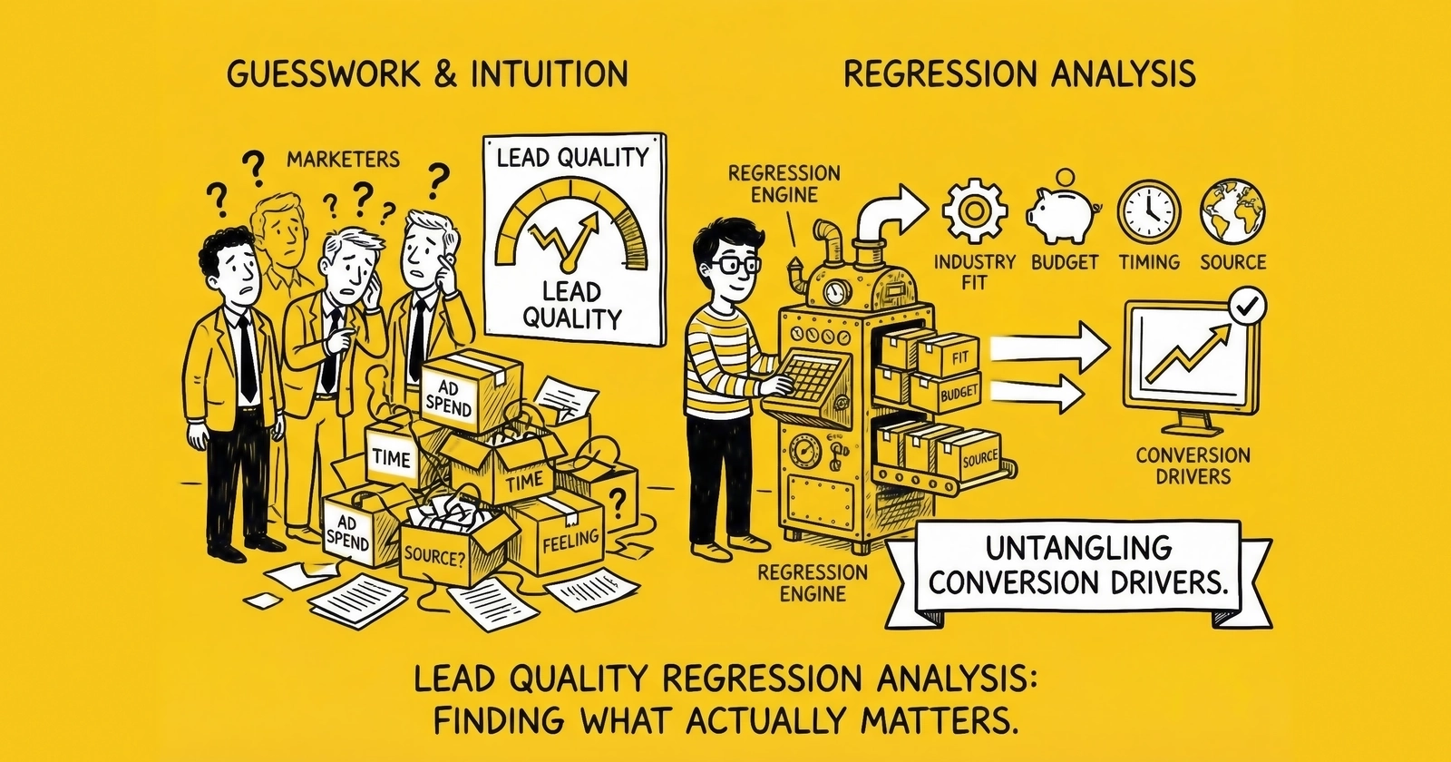
The remaining 80% hides in patterns too complex for human intuition to detect. The interaction between time of day and traffic source. The relationship between form completion speed and purchase intent. The correlation between geographic location and buyer capacity. These signals exist in your data, but you cannot see them without the right analytical tools.
Regression analysis reveals these hidden patterns. It transforms your historical lead data into predictive models that score new leads before routing, identify the variables that actually drive conversion, and optimize acquisition spending toward sources that deliver genuine quality rather than superficial validation.
This article provides a comprehensive guide to building and implementing lead quality regression models. You will learn the statistical fundamentals, identify the variables that matter most, construct models that predict real outcomes, interpret results for business decisions, and validate predictions through rigorous A/B testing. Those who master these techniques gain a substantial competitive advantage: they pay for leads that convert while competitors waste budget on leads that merely look good.
The Fundamentals of Regression Analysis for Lead Quality
Regression analysis quantifies relationships between variables. In lead generation, the core question is straightforward: which characteristics of a lead predict whether it will convert into a customer?
The simplest form, linear regression, models the relationship between one or more input variables (predictors) and a continuous output variable. But lead conversion is binary: the lead either converts or it does not. This requires logistic regression, which predicts the probability of a categorical outcome.
Why Logistic Regression for Lead Quality
Logistic regression is the workhorse of lead quality modeling for several reasons:
Binary outcomes. Lead conversion is yes or no. The consumer purchased or did not. The appointment was set or was not. Logistic regression handles this naturally, outputting probabilities between 0 and 1.
Interpretable coefficients. Unlike black-box machine learning models, logistic regression produces coefficients you can interpret. A coefficient of 0.3 for “mobile phone” means leads with mobile numbers are more likely to convert, holding other factors constant. This interpretability matters when explaining model decisions to stakeholders or debugging unexpected results.
Relatively low data requirements. While machine learning models often require millions of records, logistic regression can produce useful predictions with thousands of leads. A medium-sized operation generating 5,000-10,000 monthly leads accumulates sufficient training data within a quarter.
Regulatory defensibility. In industries facing compliance scrutiny, explainable models matter. You can document exactly why a lead received a particular score, which factors contributed, and how those factors were weighted. This transparency becomes valuable if your scoring ever faces legal challenge.
The Basic Model Structure
A lead quality regression model takes the form:
P(Conversion) = f(Lead Attributes + Source Attributes + Behavioral Signals + Timing Factors)
Where P(Conversion) is the probability that a lead will convert to a customer, and the right side includes all variables that might predict that outcome.
The model learns from historical data where you know both the lead attributes at capture time and the eventual outcome (converted or not). It identifies which combinations of attributes correlate with higher conversion probability, then applies those learned relationships to score new leads before you know their outcome.
What Regression Analysis Reveals
Beyond individual lead scores, regression analysis provides strategic insight:
Variable importance. Which factors actually predict conversion versus which factors you assumed mattered but do not? many practitioners discover their intuitions about quality are wrong. That “premium” traffic source might deliver leads that look good but convert poorly.
Interaction effects. How do variables combine? Perhaps mobile leads convert well from Facebook but poorly from Google Search. Perhaps morning leads convert well in the West but poorly in the East. Regression models capture these interactions that aggregate metrics miss.
Marginal effects. How much does each factor contribute? If improving contact rate by 10 percentage points increases conversion probability by 8%, you can calculate the ROI of contact rate improvement initiatives.
Diminishing returns. At what point does optimization hit limits? Perhaps leads contacted within 1 minute convert at 12%, leads contacted within 5 minutes convert at 10%, but leads contacted within 30 seconds show no improvement over 1 minute. Regression analysis identifies where additional investment stops paying off.
Key Variables That Drive Lead Quality and Conversion
Building an effective regression model requires identifying the right input variables. Based on analysis of millions of leads across major verticals, certain variable categories consistently predict conversion.
Consumer Intent Signals
Intent signals capture how strongly the consumer wants to purchase versus how passively they encountered your offer.
Form completion time. Leads who spend 45-90 seconds completing a form typically convert at higher rates than those who complete in under 15 seconds (bot or incentivized traffic) or over 5 minutes (distracted or uncertain consumers). Research indicates that form completion patterns correlate with conversion rates, with deliberate but efficient completion indicating genuine intent.
Question responses. Self-reported purchase timeline strongly predicts conversion. A consumer selecting “within 30 days” converts at 2-3x the rate of one selecting “just researching.” Credit score self-reports, budget ranges, and specific need descriptions all carry predictive power.
Traffic source intent. Search traffic from high-intent keywords (e.g., “best auto insurance rates today”) converts better than social media traffic from interest-based targeting. The consumer actively seeking solutions differs from the consumer interrupted by an ad.
Return visitor status. Leads from consumers who visited multiple times before converting often show higher intent than first-visit conversions. They researched, compared, and returned to act.
Contact Information Quality
Validation is necessary but not sufficient. Quality extends beyond pass/fail.
Phone line type. Mobile phones show 15-25% higher contact rates than landlines in most verticals. Consumers carry mobile phones constantly and answer unfamiliar numbers more frequently. VoIP numbers may indicate tech-savvy consumers or disposable contact information, depending on context.
Email domain. Leads with personal email domains (Gmail, Yahoo, Outlook) typically outperform business emails for consumer verticals, while the reverse holds for B2B. Disposable email domains (mailinator, guerrillamail) predict near-zero conversion.
Address verification depth. Basic address validation catches format errors. CASS-certified validation confirms deliverability. Property-appended data (homeownership, home value, year built) provides qualification signals for home-related verticals.
Phone carrier reputation. Certain carriers and number patterns correlate with higher fraud or lower contact rates. Pre-paid carrier numbers may indicate different demographics than major carrier post-paid numbers.
Source and Channel Attributes
Where leads come from predicts where they go.
Traffic source. Conversion rates vary dramatically by source. Organic search leads often convert at 2-3x the rate of paid social leads in many verticals. Affiliate leads vary widely based on affiliate quality. Direct traffic indicates existing awareness. Each source carries implicit quality signals.
Campaign type. Brand campaigns capture consumers already interested in your specific company, yielding higher conversion. Non-brand campaigns capture category interest that requires more persuasion.
Creative messaging. Leads generated by price-focused creative (“Lowest Rates Guaranteed”) may convert differently than those from value-focused creative (“Comprehensive Coverage”). The promise that attracted them shapes their expectations.
Landing page. Different pages attract different consumers. A comparison page attracts active shoppers; an educational page attracts early-stage researchers. Multi-step forms filter intent more effectively than single-page captures.
Behavioral and Temporal Variables
When and how consumers engage provides signal.
Time of day. Conversion rates vary by hour. Leads generated during business hours often convert better than late-night leads, though patterns vary by vertical. Insurance leads submitted at 2 AM may represent different intent than those submitted at 10 AM.
Day of week. Monday leads may convert differently than Friday leads. Weekend leads often show higher intent in consumer verticals, as consumers dedicate personal time to research.
Seasonality. Tax season affects financial verticals. Open enrollment affects Medicare. Summer affects solar. Seasonal patterns must be captured or they confound other variables.
Device type. Mobile leads convert differently than desktop leads in many verticals. Mobile indicates certain demographics and browsing contexts; desktop indicates others.
Buyer and Distribution Variables
Quality is relative to buyer capacity.
Buyer match score. How well does this lead match the buyer’s stated preferences? A lead outside the buyer’s target geography may be valid but low-quality for that specific buyer.
Buyer capacity utilization. Buyers at capacity may rush leads, reducing conversion. Leads distributed to buyers with available capacity often receive better treatment and convert at higher rates.
Competitive exposure. Was this lead sold exclusively or shared? Shared leads face competition; exclusive leads receive full attention. Exclusive leads typically convert at 1.5-2x the rate of shared leads, according to industry benchmarks.
Speed to contact. How quickly did the buyer contact the lead? Research consistently shows leads contacted within one minute convert at 391% higher rates. By 30 minutes, the window largely closes. Speed itself becomes a quality variable when analyzing post-distribution outcomes.
Building Your Lead Quality Regression Model
Moving from concept to implementation requires structured methodology. Here is the process that converts raw data into predictive power.
Step 1: Data Preparation and Cleaning
Regression models are only as good as their input data. Poor data quality corrupts coefficients and destroys predictive accuracy.
Assemble your dataset. Pull historical leads with known outcomes. You need the lead attributes captured at generation time plus the eventual outcome (converted/not converted, or revenue generated). Ideally, include 6-12 months of data to capture seasonal patterns. Minimum viable sample sizes range from 5,000-10,000 leads, though more data improves model stability.
Handle missing values. Leads with missing fields require decisions. Options include:
- Exclude leads with missing critical variables (reduces sample size)
- Impute missing values using median or mode (introduces assumptions)
- Create “missing” as a category for categorical variables (preserves information)
- Use multiple imputation for sophisticated handling
Document your choices. Different handling approaches can meaningfully change model results.
Remove outliers. Extreme values distort regression coefficients. A single lead with a $50,000 transaction value in a dataset averaging $500 will skew results. Identify and handle outliers through capping, transformation, or exclusion.
Address class imbalance. If only 3% of leads convert, your model may simply predict “no conversion” for everything and achieve 97% accuracy while being useless. Techniques include oversampling converted leads, undersampling non-converted leads, or using SMOTE (Synthetic Minority Oversampling Technique). Alternatively, optimize for metrics beyond accuracy, like AUC-ROC.
Step 2: Feature Engineering
Raw data rarely enters models directly. Feature engineering transforms raw inputs into model-ready predictors.
Create derived variables. Instead of raw timestamp, create:
- Hour of day (0-23)
- Day of week (1-7)
- Weekend indicator (binary)
- Business hours indicator (binary)
- Days until month end
Encode categorical variables. Regression requires numerical inputs. Encoding approaches include:
- One-hot encoding: Create binary columns for each category (State = CA becomes is_CA = 1, is_TX = 0, etc.)
- Target encoding: Replace categories with their mean conversion rate (risky due to data leakage)
- Ordinal encoding: Assign numerical order to ordered categories
Normalize continuous variables. Variables on different scales (age in years, income in dollars) can distort coefficient interpretation. Standardization (subtract mean, divide by standard deviation) puts all variables on comparable scales.
Create interaction terms. If you suspect two variables interact (source X timing), create explicit interaction features. An interaction term source_facebook:hour_evening captures whether Facebook leads perform differently in evening hours.
Step 3: Model Training and Validation
With prepared data, you can build and validate the model.
Split your data. Never evaluate a model on the same data used to train it. Standard practice:
- Training set (60-70%): Used to fit model coefficients
- Validation set (15-20%): Used to tune model parameters
- Test set (15-20%): Held out entirely until final evaluation
Alternatively, use k-fold cross-validation, which rotates through different train/test splits and averages results.
Fit the logistic regression. Using your statistical software of choice (Python’s scikit-learn, R’s glm, or dedicated platforms), fit the model to training data. The algorithm will estimate coefficients that best separate converting from non-converting leads.
Select variables. Not every variable belongs in the final model. Techniques include:
- Stepwise selection: Iteratively add or remove variables based on statistical significance
- Regularization (LASSO, Ridge): Penalize model complexity, shrinking weak coefficients toward zero
- Domain expertise: Include variables you know matter, even if marginally significant
A model with 15 meaningful variables typically outperforms one with 100 weakly predictive variables.
Tune hyperparameters. Logistic regression has few hyperparameters, but regularization strength matters. Use validation data to select the regularization level that maximizes predictive performance without overfitting.
Step 4: Model Evaluation
How well does the model actually predict?
Accuracy measures overall correct predictions, but misleads with imbalanced data. A 95% accuracy model that simply predicts “no conversion” for everything is useless.
AUC-ROC (Area Under the Receiver Operating Characteristic Curve) measures the model’s ability to distinguish converters from non-converters across all threshold levels. AUC of 0.5 indicates random guessing; 0.7-0.8 indicates acceptable discrimination; above 0.8 indicates strong predictive power. Lead quality models typically achieve AUC between 0.65-0.80, depending on vertical and data quality.
Precision and Recall trade off with each other. Precision measures what percentage of leads scored as “high quality” actually converted. Recall measures what percentage of actual converters were scored as high quality. Choose your optimization target based on business priorities.
Calibration measures whether predicted probabilities match actual frequencies. If the model predicts 30% conversion probability for a segment, approximately 30% should actually convert. Calibration curves reveal over- or under-confident predictions.
Lift charts show how much better the model performs than random selection. A model with 3x lift in the top decile means the highest-scored 10% of leads convert at 3x the average rate.
Step 5: Coefficient Interpretation
Understanding what the model learned matters as much as prediction accuracy.
Examine coefficient signs. Positive coefficients increase conversion probability; negative coefficients decrease it. A positive coefficient for “mobile phone” confirms mobile leads convert better.
Examine coefficient magnitudes. Larger absolute coefficients indicate stronger effects. In logistic regression, exponentiate coefficients to get odds ratios. An odds ratio of 2.0 means leads with that characteristic have twice the odds of conversion.
Examine statistical significance. P-values indicate confidence in the coefficient. P < 0.05 suggests the relationship is unlikely to be chance. But beware: statistical significance is not business significance. A highly significant coefficient that changes conversion probability by 0.1% may not justify action.
Look for surprises. Variables you expected to matter but do not, or unexpected predictors, reveal blind spots in your intuition. These surprises often provide the most valuable strategic insight.
From Model to Action: Practical Applications
A model in isolation changes nothing. Application creates value.
Real-Time Lead Scoring
The most direct application scores leads at capture, before routing or sale.
Score calculation. When a new lead arrives, extract its attributes, apply feature engineering, and run through the model to produce a conversion probability score from 0 to 1 (or scaled to 0-100 for usability).
Tiered routing. Route leads based on score:
- Score 80+: Priority routing to best buyers at premium pricing
- Score 50-79: Standard routing at standard pricing
- Score 25-49: Secondary routing at discounted pricing
- Score below 25: Further validation required or rejection
Industry benchmarks show companies using predictive lead scoring see 25% average conversion increases, with some reporting up to 45% improvement, according to research from Forrester and Aberdeen Group.
Dynamic pricing. Price leads based on predicted quality. A lead with 15% predicted conversion probability justifies higher pricing than one at 5% probability. Buyers will pay more for leads that actually convert.
Buyer matching. Different buyers have different capacity and preferences. A lead that scores poorly for Buyer A might score well for Buyer B based on geographic focus or product specialization. Score leads relative to each potential buyer.
Source Optimization
Aggregate lead scores by source to identify quality patterns.
Source quality indexing. Calculate mean predicted quality score by traffic source. A source with average predicted conversion of 12% outperforms one at 7%, even if cost-per-lead is similar.
True ROI calculation. Combine predicted quality with cost data:
True ROI = (Predicted Conversion Rate x Revenue per Conversion) / Cost per Lead
This calculation incorporates quality into ROI, preventing the common mistake of optimizing for volume at the expense of conversion.
Budget reallocation. Shift spend toward sources with higher predicted quality. A 2024 Demand Gen Report study found that 75% of businesses using AI qualification report significant improvement in lead quality and conversion rates.
Quality Threshold Enforcement
Use model scores to enforce minimum quality standards.
Reject low-quality leads. Leads below a minimum score threshold do not enter distribution. This protects buyer relationships and prevents margin destruction from returns.
Trigger enhanced validation. Mid-tier scores might trigger additional validation steps: SMS verification, email confirmation, or AI pre-qualification calls. These steps either upgrade the lead to acceptable quality or confirm rejection.
Compliance gating. High-risk leads (those with patterns associated with fraud or consent issues) can be flagged for enhanced documentation review before sale.
Buyer Performance Analysis
Score incoming leads and compare to buyer-reported outcomes.
Quality-adjusted conversion rates. A buyer converting 8% of leads with average predicted quality of 10% is underperforming. A buyer converting 6% of leads with average predicted quality of 4% is overperforming. Quality adjustment reveals true buyer capability.
Identify contact rate issues. If high-scored leads show low contact rates with specific buyers, the problem is buyer execution, not lead quality. This insight supports buyer coaching and negotiation.
Detect quality drift. Monitor whether the quality of leads reaching each buyer changes over time. Declining scores may explain declining conversion before the buyer complains.
A/B Testing for Model Validation
Models must prove themselves in the real world. A/B testing validates that model predictions translate into actual performance improvement.
Designing Valid Tests
Random assignment. Leads must be randomly assigned to test and control groups. Any systematic difference (routing high-volume hours to test, low-volume to control) invalidates results.
Sufficient sample size. Statistical power calculations determine required sample size. For typical lead generation conversion rates (5-15%), you need thousands of leads per variant to detect meaningful differences. Testing for 2 weeks with 500 leads per group produces noise, not insight.
Clear success metrics. Define primary metrics before the test begins. Conversion rate is typical, but consider secondary metrics: contact rate, time to conversion, revenue per lead, return rate.
Single variable testing. Change one thing at a time. If you simultaneously change scoring thresholds and routing logic, you cannot attribute outcome differences to either change specifically.
Test Structures for Lead Quality Models
Champion/Challenger testing. Route 80-90% of leads using your current approach (champion). Route 10-20% using the new model-driven approach (challenger). Compare outcomes.
Holdback testing. Score all leads but only use scores for routing on 50% of traffic. The other 50% routes as if unscored. Compare conversion rates between scored and unscored groups.
Threshold testing. Apply different score thresholds to different randomly assigned groups. Group A rejects leads below 25; Group B rejects below 35; Group C rejects below 45. Identify the optimal threshold that balances quality and volume.
Buyer randomization. For the same lead population, randomly assign to different buyer groups. Hold lead quality constant; isolate buyer performance differences.
Interpreting Test Results
Statistical significance. A result is significant if unlikely to occur by chance. Standard threshold is p < 0.05, meaning less than 5% probability the observed difference is random. But significance alone is not sufficient.
Practical significance. A statistically significant 0.3% conversion rate improvement may not justify the operational complexity of model implementation. Define minimum meaningful effect sizes before testing.
Confidence intervals. Rather than single point estimates, report ranges. “Model-driven routing improved conversion by 2.1% (95% CI: 1.4% to 2.8%)” is more honest than “conversion improved 2.1%.”
Segment analysis. Overall results may mask segment differences. The model might improve conversion for high-volume sources but hurt it for low-volume sources. Examine results by source, geography, and other relevant dimensions.
Common Testing Pitfalls
Sample contamination. If leads in test and control groups interact (same consumer submitted twice, routed differently), results are invalid.
Time-based confounding. Running test in December and control in January confounds treatment effect with seasonal effects. Run concurrent tests.
Novelty effects. New processes sometimes show temporary improvements that fade as operators adjust. Run tests long enough to capture steady-state performance.
Winner’s curse. With many tests, some will show significant results by chance. Confirm important findings with replication.
Advanced Regression Techniques
As operations mature, advanced techniques provide additional lift.
Multiple Model Approaches
Vertical-specific models. A single model across insurance, mortgage, and solar misses vertical-specific patterns. Build separate models for each vertical, training on vertical-specific outcome data.
Stage-specific models. Different models for different funnel stages:
- Top-of-funnel model predicts contact likelihood
- Mid-funnel model predicts engagement quality
- Bottom-funnel model predicts conversion probability
Multiplying probabilities across stages yields end-to-end conversion prediction.
Buyer-specific models. If different buyers have different conversion patterns, build models specific to each buyer. A lead that predicts poorly for Buyer A might predict well for Buyer B.
Regularization and Feature Selection
LASSO regression. L1 regularization shrinks weak coefficients to exactly zero, performing automatic feature selection. The result is simpler models with fewer variables, reducing overfitting risk.
Ridge regression. L2 regularization shrinks coefficients toward zero without eliminating them entirely. This handles multicollinearity (correlated predictors) better than standard logistic regression.
Elastic net. Combines L1 and L2 regularization, capturing benefits of both. Particularly useful when you have many potential predictors and want automatic selection.
Ensemble Methods
Random forests. Build many decision trees on random subsets of data and average predictions. Random forests often outperform logistic regression in raw predictive accuracy, though they sacrifice interpretability.
Gradient boosting. Sequentially build models that correct errors of previous models. XGBoost and LightGBM are popular implementations. These methods frequently achieve the best predictive performance in machine learning competitions.
Model stacking. Use predictions from multiple models as inputs to a meta-model. Combine logistic regression, random forest, and gradient boosting predictions to capture different pattern types.
The trade-off: ensemble methods provide better prediction but less interpretability. For operations prioritizing explainability (compliance-sensitive verticals, stakeholder communication), simpler models may be preferable despite slightly lower accuracy.
Model Monitoring and Maintenance
Models degrade over time. Market conditions change, traffic sources evolve, and buyer behaviors shift.
Monitor prediction accuracy. Track actual versus predicted conversion rates weekly. Divergence indicates model drift.
Retrain periodically. Quarterly retraining on recent data captures evolving patterns. Include the most recent 6-12 months of data to balance recency with sample size.
Monitor feature distributions. If a key predictor’s distribution changes dramatically (a traffic source suddenly shifts demographics), model predictions may become unreliable.
Establish retraining triggers. Define automatic retraining when:
- AUC drops below 0.65
- Predicted and actual conversion rates diverge by more than 20%
- New major traffic sources represent more than 15% of volume
- Seasonal factors require updated coefficients
Implementation Considerations
Data Infrastructure Requirements
Effective regression analysis requires data infrastructure that many lead generation operations lack.
Lead-level data warehouse. You need every lead with every attribute and eventual outcome in a queryable format. Spreadsheets fail at scale. SQL databases or cloud data warehouses (BigQuery, Snowflake, Redshift) provide the necessary capability.
Outcome tracking. You must connect leads to conversion outcomes. This requires either buyer feedback integration, CRM disposition data, or conversion pixel tracking. Without outcome data, you cannot train or validate models.
Real-time scoring capability. To score leads before routing, you need infrastructure that can execute model predictions in milliseconds. This typically requires model deployment platforms or embedded scoring in your lead distribution system.
Team Capabilities
Building and maintaining regression models requires specific skills:
Statistical knowledge. Someone must understand logistic regression mechanics, validation approaches, and interpretation pitfalls. This might be a data scientist, quantitative analyst, or trained marketing analyst.
Data engineering. Converting raw data into model-ready features requires SQL proficiency, ETL pipeline management, and data quality monitoring.
Business context. Statistical outputs require business interpretation. Domain experts must translate coefficient changes into operational decisions.
For smaller operations, consider:
- Training existing analysts in regression techniques (courses available through Coursera, DataCamp, university extensions)
- Consulting engagements for initial model development with knowledge transfer
- Platform solutions that embed scoring without requiring custom model building
Platform Options
Several platforms provide lead scoring capabilities without requiring in-house model building:
Lead distribution platforms. Major platforms like boberdoo, LeadsPedia, and Phonexa increasingly include scoring features. These may not offer the customization of custom models but require minimal technical investment.
Marketing automation platforms. HubSpot, Marketo, and Salesforce provide lead scoring based on engagement and demographic data. These work better for B2B marketing leads than for consumer lead generation operations.
Dedicated scoring solutions. Platforms like Infer, 6sense, and MadKudu specialize in predictive lead scoring, primarily for B2B contexts.
Custom development. Python (scikit-learn, statsmodels) or R provide full control over model specification, training, and deployment. This approach requires data science capability but offers maximum flexibility.
Frequently Asked Questions
What is lead quality regression analysis?
Lead quality regression analysis uses statistical models to identify which lead characteristics predict conversion to customers. The analysis examines historical leads with known outcomes, identifies patterns distinguishing converters from non-converters, and applies those patterns to score new leads before you know their outcome. Logistic regression is the most common technique, producing probability scores between 0 and 1 that indicate conversion likelihood.
How much historical data do I need to build a regression model?
A minimum of 5,000-10,000 leads with known conversion outcomes provides a viable starting point. Larger datasets (50,000+ leads) produce more stable models and enable detection of subtle patterns. You also need sufficient conversions in your data; with a 5% conversion rate, 10,000 leads yield only 500 conversion examples, which limits model complexity. Aim for at least 500-1,000 positive outcomes (conversions) in your training data.
What variables matter most for predicting lead conversion?
The most consistently predictive variables across verticals include: traffic source intent (search outperforms social), speed to contact (within 1 minute optimal), consumer self-reported timeline and need specificity, phone line type (mobile outperforms landline), and form completion behavior (deliberate completion signals genuine intent). However, the specific predictors that matter most vary by vertical, buyer, and business model. Model building reveals which variables matter in your specific context.
How do I implement lead scoring in real-time?
Real-time scoring requires: (1) a trained model exported in a deployable format, (2) infrastructure to capture lead attributes at submission, (3) feature engineering logic to transform attributes into model inputs, and (4) scoring logic that executes model predictions in milliseconds. Lead distribution platforms increasingly support embedded scoring. Custom implementations typically use API-based model serving (Flask, FastAPI, or cloud ML services) integrated with your lead capture forms.
What is a good AUC score for a lead quality model?
AUC (Area Under the ROC Curve) measures model discrimination ability. For lead quality models, AUC between 0.65-0.75 indicates acceptable prediction; 0.75-0.85 indicates strong prediction; above 0.85 is exceptional but rare. An AUC of 0.70 means that if you randomly select one converting lead and one non-converting lead, the model will correctly rank them 70% of the time. Most production lead quality models achieve AUC in the 0.68-0.78 range.
How often should I retrain my lead quality model?
Quarterly retraining balances model freshness against operational overhead. More frequent retraining (monthly) is warranted when: traffic sources change rapidly, market conditions shift significantly, or you detect model drift through monitoring. Establish automatic retraining triggers based on prediction accuracy degradation (e.g., retrain when AUC drops below threshold or predicted/actual conversion rates diverge by more than 20%).
What is the difference between lead scoring and lead validation?
Lead validation confirms data accuracy: the phone number connects, the email delivers, the address exists. Validation is binary and occurs in milliseconds. Lead scoring predicts conversion probability: given a validated lead, how likely is this consumer to become a customer? Scoring considers intent signals, source quality, timing, and buyer match. Validation is necessary but not sufficient; many validated leads never convert. Scoring separates high-potential leads from low-potential leads among the validated population.
How do I know if my regression model is working?
Validate model performance through: (1) holdout testing, where you evaluate predictions on data the model never saw during training; (2) lift analysis, confirming that high-scored leads convert at meaningfully higher rates than low-scored leads; (3) calibration checks, verifying that predicted probabilities match actual conversion frequencies; and (4) A/B testing, comparing business outcomes when using model-driven routing versus baseline routing. A working model shows clear score-stratified conversion differences and improves business metrics in controlled tests.
Can regression analysis detect lead fraud?
Regression models can identify patterns associated with fraud, such as: unusually fast form completion, suspicious browser or device characteristics, known problematic IP ranges, and behavioral anomalies. However, fraud detection typically requires specialized models trained specifically on fraud outcomes rather than conversion outcomes. Some fraud patterns that reduce conversion (bot traffic) will surface in quality models, but sophisticated fraud designed to pass validation and initial contact requires dedicated fraud scoring.
What should I do if my model shows unexpected results?
Unexpected results reveal either model problems or genuine surprises in your data. Investigate systematically: (1) verify data quality for the surprising variables, (2) check for data leakage where outcome information inappropriately entered predictors, (3) examine sample sizes for the relevant segments, and (4) validate the pattern in holdout data. If the pattern persists through verification, you have discovered something genuine about your market that contradicts your assumptions. These surprises often provide the most valuable strategic insights.
Key Takeaways
Regression analysis reveals hidden quality drivers. Human intuition captures perhaps 20% of what determines lead quality. Statistical models identify the remaining 80% hidden in variable interactions, timing patterns, and source-level differences that aggregate metrics obscure.
Logistic regression is the workhorse model. For lead quality prediction, logistic regression provides the ideal balance of predictive power, interpretability, and reasonable data requirements. More complex methods may improve accuracy marginally but sacrifice explainability.
The right variables matter more than sophisticated methods. Intent signals (form completion behavior, purchase timeline, traffic source), contact quality (phone type, email domain), and timing factors (hour, day, seasonality) consistently predict conversion. Include these variable categories in any lead quality model.
Model validation requires A/B testing. Statistical validation on holdout data confirms model accuracy. But business validation requires A/B testing in production, comparing outcomes when using model-driven decisions versus baseline approaches. Only production testing proves that statistical accuracy translates into business improvement.
Companies using predictive lead scoring see 25%+ conversion improvements. Research consistently shows that organizations implementing lead scoring based on predictive models achieve substantially higher conversion rates, shorter sales cycles, and better marketing ROI than those treating all leads equally.
Models require ongoing maintenance. Market conditions, traffic sources, and buyer behaviors evolve. Models trained on historical data degrade over time. Quarterly retraining and continuous monitoring prevent model drift from eroding prediction accuracy.
Data infrastructure is foundational. Lead-level data warehousing, outcome tracking, and real-time scoring capability require infrastructure investment. Without proper data foundation, model building produces one-time analysis rather than operational improvement.
Start simple and iterate. Begin with a basic model on core variables. Validate it works. Then add complexity: more variables, advanced techniques, ensemble methods. Incremental improvement beats elaborate systems that never deploy.
Lead quality regression analysis transforms data into competitive advantage. Those who build these capabilities score leads more accurately, route more effectively, and allocate budgets toward sources that deliver genuine conversion rather than superficial validation. In a market where margins compress and quality increasingly determines survival, statistical rigor separates professionals from amateurs.