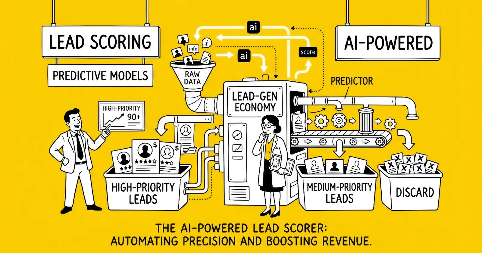
The failure mode for lead scoring projects is not building a model that underperforms. It is building a model that performs well on historical data, passes validation, gets deployed to production, and then fails to improve conversion because the fundamental data problems were never addressed.
Most lead scoring projects skip the foundational questions: What data is actually predictive? How much of it is available at the time of scoring? Is the training data labeled correctly? Are the outcome definitions precise enough to train toward? These questions are more important than algorithm selection or model architecture choices, which most practitioners spend disproportionate time debating.
This guide covers the technical implementation path from raw lead data to a deployed, maintained scoring model. The sequence matters: data problems must be solved before model development begins, and deployment architecture must be understood before choosing between real-time and batch approaches. The goal is a scoring system that produces probability estimates that meaningfully separate leads likely to convert from those unlikely to – and that continues producing accurate estimates as data distributions shift over time.
Defining the Scoring Objective
Before writing any code or auditing any data, define precisely what the model will predict. This decision determines everything that follows.
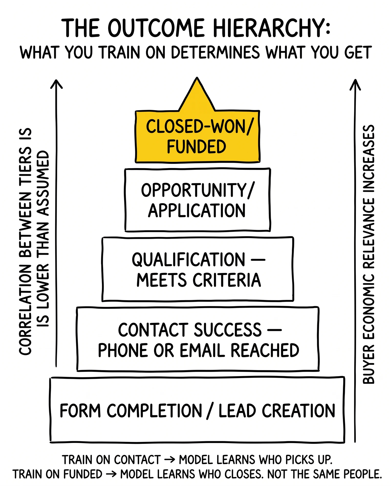
The Outcome Hierarchy Problem
A lead conversion does not have a single definition. Most organizations have at least five distinct outcomes they could predict:
- Form completion / lead creation – the consumer submitted contact information
- Contact success – a sales representative reached the consumer by phone or email
- Qualification – the consumer met minimum product criteria (credit score, geography, intent)
- Opportunity / application – the consumer moved forward in the sales process
- Closed-won / funded – the transaction completed
Models trained on different outcome definitions produce different scores, and the correlation between these stages is lower than most practitioners assume. A lead likely to convert to phone contact is not necessarily likely to convert to a funded loan. A lead likely to qualify is not the same set as a lead likely to eventually close.
Choosing the right outcome:
The scoring objective should match the operational decision the score will support:
- If the score routes which leads get called first, optimize for contact rate or qualification rate
- If the score determines which leads receive human follow-up versus automated nurture, optimize for opportunity creation
- If the score informs lead pricing or buyer routing, optimize for the outcome that most directly affects buyer economics (usually funded loan or closed sale)
One common mistake: training on contact rate because contact data is available immediately, but deploying the score in contexts where funded loan rate is the relevant metric. The model will learn to identify leads that pick up the phone, not leads that close – which are different populations.
Defining the Observation and Outcome Windows
Two time windows require explicit definition:
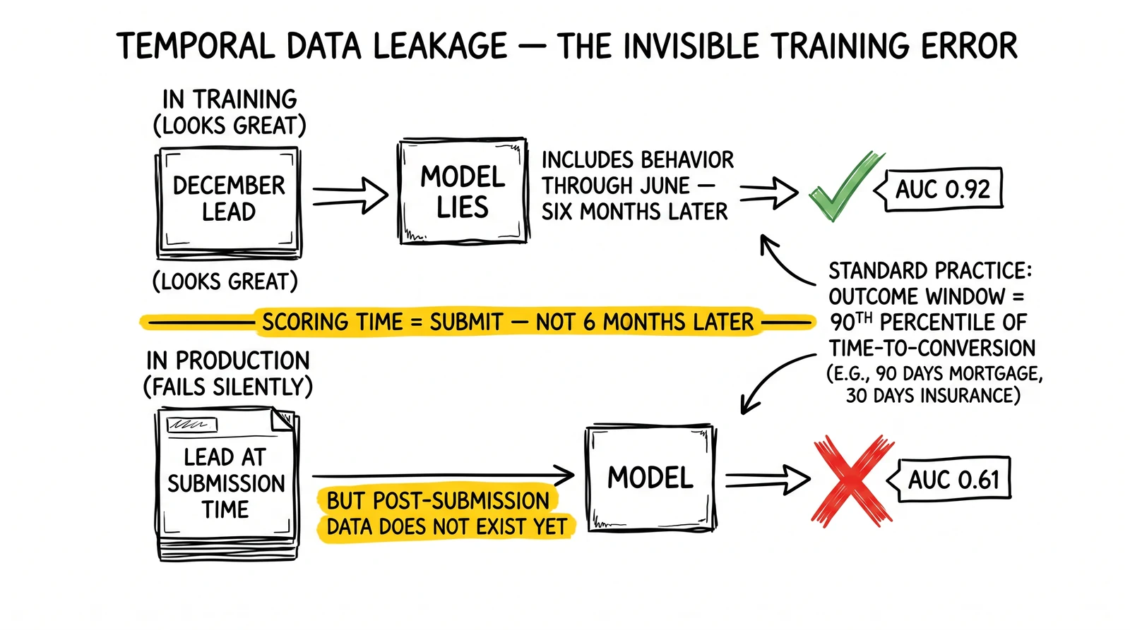
Observation window: The period of data collection for each lead. Feature values should reflect information available at the time of scoring, not information accumulated afterward. If you score leads at submission, behavioral data from after submission cannot be a feature – it does not exist yet at scoring time.
This distinction matters for training data construction. If you pull a lead from December and include all behavioral data through June for training, you have included six months of post-submission behavior as features. The model will learn from this future data, appear to validate well, and then fail in production because post-submission behavior is not available at scoring time. This is called temporal data leakage and is the most common training error in lead scoring implementations.
Outcome window: How long after lead creation you wait before labeling the outcome. If the sales cycle averages 60 days, leads created in the last 60 days of your training dataset have not had time to convert – they will be labeled as non-conversions even if they eventually will convert. Including these leads biases the model toward underpredicting for recent leads.
Standard practice: define outcome window equal to the 90th percentile of the time-to-conversion distribution. For mortgage leads, this might be 90-120 days. For insurance leads, 30-45 days. Exclude leads created within the outcome window from training data.
Data Inventory and Predictive Field Assessment
Before feature engineering, audit what data exists, when it becomes available, and whether it predicts conversion in practice. Most lead data ecosystems contain fields with zero predictive value alongside fields that carry strong signal that gets overlooked.
Lead Attribute Fields: What Actually Predicts
Not all form fields predict conversion equally. The following categories appear consistently across lead verticals:
Phone number quality signals:
- Phone line type (mobile vs. landline vs. VoIP) – VoIP numbers show systematically lower contact rates across most verticals
- Phone validation status (connected, disconnected, invalid format) – disconnected phones predict zero conversion by definition
- Phone carrier – certain carriers correlate with specific geographic or demographic patterns
- Country code and area code – geographic validation beyond what self-reported ZIP provides
Email quality signals:
- Email domain type (personal Gmail/Yahoo vs. corporate domain vs. disposable) – disposable email domains near-perfectly predict non-conversion for long-cycle sales
- Email deliverability status (valid syntax, MX record exists, inbox active) – undeliverable emails cannot be nurtured
- Email domain age – very new domains correlate with fraud in many verticals
Form completion behavior:
- Time to complete (seconds from first field interaction to submit) – both very fast (bots) and very slow (confusion) predict lower conversion
- Field revision count – leads that retype fields multiple times may have lower commitment to accuracy
- Form abandonment and return – a lead who started, abandoned, and returned converted to complete shows different intent than one who completed in a single pass
Self-reported data quality:
- Consistency between related fields (ZIP code matching stated city and state)
- Plausibility of self-reported values (annual income of $1M for a stated occupation of “student”)
- Specificity of open-text fields – leads who write specific, detailed answers to optional fields show different engagement than those who enter single characters
Behavioral Features: Timing and Sequence
Behavioral data accumulated before form submission often provides the highest predictive lift, but it requires proper tracking infrastructure to capture. Key behavioral categories:
Pre-submission site behavior:
- Pages viewed and sequence (pricing page before comparison page signals different intent than the reverse)
- Time on site in the session and in prior sessions
- Number of visits before submission (first-visit submissions behave differently than sixth-visit submissions)
- Content categories engaged with (product-focused content vs. general informational content)
- Source and referrer (branded search terms vs. generic category terms)
Device and environment signals:
- Device type and operating system (patterns vary by vertical – mortgage leads from mobile devices convert at different rates than desktop)
- Browser and user agent (outdated browsers correlate with certain demographic patterns)
- Connection type where available (mobile data vs. WiFi has predictive value in some contexts)
- Time of day and day of week at submission
Geographic signals beyond self-reported location:
- IP geolocation versus stated location (significant discrepancies predict lower quality)
- IP address type (residential, corporate, data center/VPN)
- Distance from service area center for geographic services
What to Exclude from Features
Some data fields seem predictive during training but should be excluded:
Fields with high missing rates: Features missing in more than 30-40% of records require careful handling. If the model learns to interpret missingness as a signal, it will behave differently than expected when data availability changes.
Fields with post-submission timing: Any data collected after the submission event cannot be available at scoring time in a real-time deployment. Exclude from features or clearly limit use to batch re-scoring workflows.
Fields that proxy for protected characteristics: In regulated verticals (mortgage, insurance, employment), features that closely proxy for protected characteristics (race, gender, age) create fair lending or anti-discrimination exposure. Phone area codes that strongly correlate with demographic composition, for example, require careful evaluation before use.
Personally identifying information: Raw names, email addresses, and phone numbers should not be used as model features. Their predictive value (if any) should be extracted through derived features (email domain type, phone line type) that do not expose PII in the model.
Feature Engineering for Lead Data
Feature engineering transforms raw field values into model inputs that reveal underlying patterns. This step consistently produces more prediction lift than algorithm selection.
Encoding Categorical Variables
Most lead data contains categorical fields that cannot be fed to most machine learning algorithms in raw form: state names, traffic sources, lead categories, service types. Several encoding strategies apply:
One-hot encoding creates a binary column for each category value. “State: Texas” becomes a column state_texas with value 1 for Texas leads and 0 for all others. Works well for low-cardinality fields (fewer than 20 categories). Creates dimensionality problems for high-cardinality fields (hundreds of ZIP codes, thousands of city names).
Target encoding replaces each category value with the average conversion rate for that category in training data. “State: Texas” might encode as 0.038 if Texas leads convert at 3.8% in training data. Works well for high-cardinality fields without creating dimensionality problems. Requires care to avoid overfitting – leave-one-out cross-validation during encoding prevents leakage.
Frequency encoding replaces each category with its frequency in training data. Less information-rich than target encoding but useful when conversion rates by category are unstable or too sparse to estimate reliably.
Embeddings (learned vector representations) work well when category relationships have meaningful structure – for example, adjacent ZIP codes share geographic characteristics. Embeddings require more sophisticated infrastructure and larger datasets.
For typical lead scoring applications: use one-hot encoding for fields with fewer than 15 values, target encoding for high-cardinality fields (states, ZIP codes, traffic sources), and experiment with embeddings only if gradient boosting with target encoding shows evidence of ceiling performance.
Temporal Feature Construction
Time-based features deserve specific attention because timing signals are often among the strongest predictors in lead scoring and are frequently left as raw timestamps rather than engineered into predictive signals.
From a submission timestamp, extract:
- Hour of day (0-23, cyclically encoded using sin/cos to preserve hour adjacency)
- Day of week (0-6, cyclically encoded)
- Week of month (1-5)
- Month (1-12, cyclically encoded)
- Day of year (proximity to seasonal patterns)
- Days since campaign launch (for time-limited offers)
- Days until end of period (month-end, quarter-end urgency)
- Whether submission occurred during business hours (contextualizes intent for B2B)
- Whether submission occurred on a holiday or holiday-adjacent day
Cyclical encoding for periodic variables prevents the model from treating hour 23 and hour 0 as maximally distant (they are adjacent). Encode as:
hour_sin = sin(2π × hour / 24)
hour_cos = cos(2π × hour / 24)
From behavioral session data:
- Time between sessions (recency of last visit)
- Rate of engagement change (increasing vs. decreasing session frequency)
- Time between first and last touch before submission
Interaction Features
Machine learning algorithms discover interactions automatically, but explicitly constructing interaction features for domain-knowledge-driven combinations can accelerate learning and reduce the training data required.
Useful interaction constructions for lead data:
phone_valid × email_valid– both valid suggests higher quality than either alonesession_count × time_on_site– engagement volume (more visits × more time = higher investment)page_views_pricing × days_since_first_visit– deliberate consideration (multiple pricing views over time)lead_source_type × device_type– certain source-device combinations have systematic quality differences
Construct interactions based on domain hypotheses first, then validate that they improve held-out performance. Interactions that do not improve performance on holdout data should be removed – they may reflect training data patterns rather than generalizable signals.
Handling Missing Values
Missing values require explicit handling decisions; most algorithms cannot process null values natively:
Imputation with mean/median: Replace numeric missing values with the training data mean or median. Appropriate when missing values are random and the field has high coverage (under 10% missing).
Imputation with sentinel values: Replace missing values with a value outside the natural range (e.g., -1 for a field that is always 0-100). This tells tree-based models “this record had missing data,” which can be predictive information. Effective when missingness itself carries signal.
Separate missingness indicator: Add a binary feature field_X_missing alongside the imputed value. This allows the model to learn both the imputed value’s effect and the effect of the field being missing. Useful when you suspect missingness is informative but are uncertain.
Exclusion: For fields with more than 40% missing rate, consider excluding the field entirely unless missingness itself is highly predictive. High-missing-rate fields add noise and can destabilize models.
Model Selection: Architecture Choices by Dataset Size
Dataset size significantly constrains which model architectures are appropriate. Sophisticated models that outperform on large datasets underperform on small datasets because they have too many parameters to estimate reliably from limited training examples.
Small Datasets (Fewer Than 5,000 Conversion Events)
With fewer than 5,000 positive examples (conversions), complex models overfit. The model memorizes training examples rather than learning generalizable patterns.
Best choices:
- Logistic regression with regularization (L1/Lasso or L2/Ridge): Interpretable, computationally lightweight, resistant to overfitting with appropriate regularization strength
- Linear SVM: Similar properties to logistic regression for binary classification
- Shallow decision trees (max depth 3-5): Interpretable, limited parameters
What to avoid:
- Deep random forests (many trees with many features per tree overfit small datasets)
- Gradient boosting with many iterations
- Any neural network approach
Practical expectation: With under 5,000 positive examples, expect modest improvement over rule-based scoring. The goal is consistency and interpretability, not maximum lift. A logistic regression model trained on 3,000 conversion events might achieve 1.5-2.0x lift in the top decile – better than random, better than simple rules, but not the 3-4x lift possible with larger datasets.
Medium Datasets (5,000-50,000 Conversion Events)
This range supports gradient boosting approaches that typically outperform linear models by capturing non-linear relationships and feature interactions automatically.
Best choices:
- LightGBM: Fast, memory-efficient, handles categorical variables natively, excellent default performance
- XGBoost: Strong established performance, good documentation and community support
- CatBoost: Particularly effective when many categorical features are present
Implementation recommendation: Start with LightGBM using default hyperparameters to establish a baseline. Then tune: learning rate, number of trees, maximum tree depth, minimum samples per leaf, and regularization parameters. Bayesian hyperparameter optimization (Optuna library is well-suited) finds good parameter combinations more efficiently than grid search.
Expected performance: 2-3x lift in the top decile with well-engineered features. Feature engineering matters more than hyperparameter tuning at this scale.
Large Datasets (More Than 50,000 Conversion Events)
Large datasets support more complex approaches but gradient boosting often remains the best choice due to its performance-to-complexity ratio.
Best choices:
- Gradient boosting (LightGBM, XGBoost, CatBoost): Still typically the top performer on tabular data
- Random forests: Useful as ensemble components, easier to parallelize
- Neural networks (shallow: 2-3 layers): Worth evaluating when features include many continuous behavioral metrics
When neural networks add value for lead scoring: Neural networks outperform gradient boosting primarily when:
- Raw behavioral event sequences need to be processed (recurrent architectures for session data)
- Text fields contain meaningful signal that benefits from language model encodings
- The dataset exceeds 500,000 positive examples, providing enough data to learn complex non-linear patterns
For most lead scoring implementations in the 50,000-200,000 positive example range, gradient boosting will match or exceed neural network performance with substantially lower implementation complexity.
Stacking and ensembles: At large scale, combining predictions from multiple model types (gradient boosting + logistic regression + random forest) through a meta-learner can improve performance by 5-10% over the best individual model. This adds operational complexity but is worth evaluating if the performance gains translate to meaningful business impact.
Validation Methodology Without Data Leakage
Validation methodology determines whether model performance estimates are reliable or illusory. Poor validation is the most common cause of models that perform well in testing and poorly in production.
The Data Splitting Decision
Standard train-test splitting randomly partitions data into training and evaluation sets. For lead scoring specifically, temporal splitting often produces more realistic performance estimates:
Random splitting: Train on 80% of data, test on 20% selected randomly. The model trains and evaluates on leads from the same time periods, potentially learning temporal patterns that do not generalize to future data.
Temporal splitting: Train on leads from months 1-12, evaluate on months 13-15. This tests whether patterns discovered in historical data predict behavior in a future period – which is the actual deployment challenge.
Walk-forward validation: Train on months 1-6, evaluate on month 7. Then train on months 1-7, evaluate on month 8. Repeat for each subsequent month. Average performance across evaluation periods. This approach provides the most realistic estimate of ongoing production performance, accounting for concept drift across time.
For most implementations, temporal splitting with a 3-6 month holdout period provides sufficient realism. Walk-forward validation adds value when lead quality or market conditions change significantly over the training period.
Calibration Testing
Model calibration measures whether probability scores reflect actual conversion rates. A well-calibrated model that predicts 30% conversion probability should actually see approximately 30% of similarly-scored leads convert.
Poor calibration means scores are directionally correct (high scores convert more than low scores) but the absolute probability values are wrong. This matters when scores are used for threshold-based decisions (call all leads above 25% probability) or economic modeling (expected revenue per lead = predicted conversion × average deal value).
Test calibration using reliability diagrams (also called calibration curves): bin leads by predicted probability, then plot actual conversion rate per bin versus predicted probability. Perfectly calibrated models produce a diagonal line; systematic over- or under-prediction shows as deviation from the diagonal.
If calibration is poor, apply Platt Scaling (logistic regression applied to raw model outputs) or Isotonic Regression as post-processing calibration steps. Both are standard techniques that correct systematic bias in probability outputs.
Performance Metrics for Operational Use
Several metrics are relevant for evaluating scoring system performance; the right metric depends on the operational question:
Lift in top decile: Of leads scored in the top 10%, how much higher is their actual conversion rate than the overall population? A 3.0x lift means top-decile leads convert at 3x the baseline rate. This metric maps directly to the value of prioritization – knowing that 3x lift is achievable determines how aggressively to act on scoring.
AUC-ROC: The probability that the model ranks a random converter above a random non-converter. AUC above 0.75 is generally useful; above 0.85 is strong for lead scoring applications. AUC measures rank ordering ability independent of any specific threshold.
Precision at K: Of the top K leads (operationally: the number your team can work in a day), what fraction converts? This metric directly answers the operational question: “if I can only call 100 leads today, what fraction will convert?”
F1 score at threshold: If operating at a specific score threshold (call all leads above 0.30), F1 balances precision and recall at that threshold. Useful when the threshold has operational significance.
Do not use accuracy as a primary metric. At 5% base conversion rate, a model that predicts “no conversion” for every lead achieves 95% accuracy while being completely useless.
Deployment Architecture: Real-Time vs. Batch Scoring
The deployment architecture choice determines latency, infrastructure cost, and what features can be included in scoring.
When Real-Time Scoring Is Required
Real-time scoring is necessary when the score will influence:
- Immediate lead routing (which buyer receives the lead within seconds of submission)
- Real-time response personalization (which offer, message, or follow-up sequence the lead receives immediately)
- Instant price optimization in ping-post systems (where the score informs the bid response within milliseconds)
Real-time requirements:
- Scoring latency under 200ms (including feature retrieval, model inference, and response)
- High availability (99.9%+ uptime) because lead flow cannot wait for a scoring service to recover
- Horizontal scalability to handle volume spikes without latency degradation
Real-time architecture components:
- Feature store: Pre-computed features stored in Redis or another low-latency key-value store, retrievable in under 10ms by lead identifier
- Real-time feature computation: Features derived from the current request (submission timestamp, form values, device fingerprint) computed within the scoring request
- Model serving: Serialized model loaded into memory (not reloaded per request), serving predictions through REST or gRPC API
- Monitoring: Latency tracking, prediction distribution tracking, error rate alerting
For most lead generation deployments, a Python service using FastAPI with the trained model loaded at startup, connected to Redis for pre-computed features, can achieve sub-100ms scoring latency at moderate traffic volumes. Cloud-managed model serving (AWS SageMaker, Google Vertex AI Prediction) adds infrastructure management burden but provides autoscaling out of the box.
When Batch Scoring Suffices
Batch scoring is appropriate when scores will be used for:
- CRM record enrichment (sales team reviews scores at start of each day)
- Lead prioritization queues (leads scored hourly and prioritized for next shift)
- Lead pricing decisions that do not need to happen in real-time
Batch scoring is simpler to implement, requires no real-time infrastructure, and allows use of features that require time to compute (multi-session behavioral aggregates, enrichment API responses that take seconds).
Batch scoring pipeline:
- Extraction: Pull new or unscored leads from source systems on schedule (every hour, every 4 hours, or nightly)
- Feature computation: Join lead data with behavioral data, compute engineered features, retrieve enrichment data
- Model inference: Apply model to batch of leads, generate probability scores
- Distribution: Write scores to CRM via API, update lead management system records, trigger workflow rules based on score thresholds
Batch processing is appropriate for most mid-market operations processing under 10,000 leads per day. The operational simplicity of batch often outweighs real-time latency advantages when the sales process itself does not require instant prioritization.
Hybrid: Initial Score Plus Behavioral Re-Scoring
Many production implementations use both patterns: real-time scoring at submission for immediate routing, plus scheduled re-scoring as behavioral data accumulates.
The initial real-time score uses only data available at submission time: form fields, device signals, source attribution, phone/email validation. This score determines initial routing and priority.
Subsequent batch re-scoring incorporates post-submission behavioral data: email open rates, website return visits, response to initial outreach. Re-scoring runs every 24-48 hours and updates CRM scores to reflect accumulated information.
This hybrid approach captures the urgency benefits of real-time scoring while improving accuracy over time as more signal accumulates.
Model Maintenance and Degradation Management
Models deployed to production degrade over time. Market conditions change, consumer behavior shifts, lead sources evolve, and validation data distributions drift from training data. Without active maintenance, a model that delivered 2.5x lift in the first month may deliver 1.3x lift twelve months later.
Monitoring for Degradation
Two categories of monitoring detect model problems:
Input monitoring tracks whether features flowing into production scoring have shifted from training-time distributions. If the fraction of mobile leads increases from 40% to 65% over six months, features derived from device type will behave differently than during training. Input drift does not guarantee performance degradation, but it signals that performance should be checked.
Output monitoring tracks whether score distributions and score-to-outcome correlations remain stable. If leads scoring above 0.70 are converting at 12% during training but 6% in production six months later, the model has degraded. Output monitoring requires outcome data with appropriate lag – in a 60-day sales cycle, you cannot evaluate score accuracy for recent leads.
Alerting thresholds: trigger review when top-decile lift falls more than 30% below initial deployment performance, or when input feature distributions shift more than 2 standard deviations from training-time means.
Retraining Schedule
Retraining frequency should reflect how quickly the underlying patterns change:
- Monthly retraining: Appropriate for most lead scoring applications where market conditions evolve moderately. Adds recent data to training while maintaining historical patterns.
- Quarterly retraining: Appropriate when sales cycles are long (3+ months) and patterns change slowly.
- Event-triggered retraining: Retrain when monitoring detects significant drift or performance degradation. More sophisticated but avoids unnecessary retraining costs.
Retraining does not always mean rebuilding from scratch. Incremental learning approaches (online learning algorithms, transfer learning from existing models) can update model weights with new data without complete retraining. For gradient boosting specifically, adding new trees to an existing ensemble can incorporate new patterns with less computational cost than full retraining.
Model Versioning and Rollback
Maintain version history for deployed models. When a new model version is deployed, preserve the ability to revert to the previous version within minutes if the new model underperforms.
A/B test new model versions against the current production model before full rollout. Route a percentage of leads through the new model version, compare conversion outcomes between routing variants over 2-4 weeks, and roll out fully only when the new version shows statistically significant improvement.
Shadow scoring – running the new model in parallel without routing consequences – provides additional safety before affecting live lead flow.
FAQ
How many leads do I need before building a scoring model?
The minimum practical threshold is approximately 1,000 positive examples (converted leads) in historical data. Below this, patterns are difficult to distinguish from noise and models will overfit. The practical minimum for a model likely to outperform simple rules significantly is 3,000-5,000 positive examples. More data improves performance, particularly for complex behavioral features, until around 100,000 positive examples where marginal returns from more data flatten.
Should the model predict a probability or a score tier?
Probability outputs (0.0-1.0) are more useful than tiered outputs (high/medium/low) because they enable threshold-based decisions based on business economics rather than arbitrary categories. The probability can be converted to tiers later if that is operationally simpler – but the underlying model should produce calibrated probabilities. Tiered outputs from the model itself discard information by collapsing continuous probability estimates into categories.
How do I handle the class imbalance problem in lead scoring?
Most lead datasets have severe class imbalance: 2-10% positive rate. The most reliable approach for gradient boosting is adjusting the class weight parameter to penalize false negatives more heavily than false positives during training. The scale_pos_weight parameter in XGBoost and LightGBM controls this. Set it to approximately (negative count / positive count). Alternative approaches (SMOTE oversampling, random undersampling) work but introduce additional complexity without consistently improving performance over class weighting.
What is temporal data leakage and how do I prevent it?
Temporal leakage occurs when training features include information that would not be available at actual scoring time. Common sources: including post-submission behavioral data in features, including outcome-correlated data collected during the sales process in features, or including aggregate statistics computed across the full dataset (including future data) in features. Prevention: explicitly document the timestamp at which each feature becomes available, and enforce that training features only use data available at the defined scoring time.
How often should the model be retrained?
Monthly retraining works for most applications. Monitor performance against outcome data on a rolling basis – if monitoring shows top-decile lift falling more than 20-30% from deployment baseline, retrain immediately. If performance remains stable, monthly retraining is typically sufficient. High-volume operations processing 50,000+ leads per day may benefit from weekly retraining because more outcome data accumulates faster.
Sources
- Hastie, Tibshirani, Friedman: “The Elements of Statistical Learning” – foundational reference on model architecture trade-offs
- Chen and Guestrin: “XGBoost: A Scalable Tree Boosting System” (KDD 2016) – foundational paper on gradient boosting implementations
- Ke et al.: “LightGBM: A Highly Efficient Gradient Boosting Decision Tree” (NeurIPS 2017) – LightGBM technical foundation
- Scikit-learn documentation: calibration, class imbalance handling, pipeline construction – scikit-learn.org
- Guo et al.: “On Calibration of Modern Neural Networks” (ICML 2017) – calibration testing methodology
- Sculley et al.: “Hidden Technical Debt in Machine Learning Systems” (NeurIPS 2015) – ML systems operational challenges
- Molnar: “Interpretable Machine Learning” – feature importance, SHAP values, model explanation methods – christophm.github.io/interpretable-ml-book/
- Forrester Research - Research foundation for B2B marketing and sales technology adoption statistics, including AI implementation rates
- Salesforce Research Reports - Industry data on sales cycle optimization and AI-driven lead prioritization outcomes
- HubSpot State of Marketing - Annual survey data on marketing technology adoption and conversion rate benchmarks
- Google Core Web Vitals - Technical specifications for real-time performance metrics including latency thresholds
- MLflow Documentation - Open-source platform documentation for model versioning, registry, and deployment patterns referenced in the article