The mortgage lead market does not respond to rate changes the way most operators assume. Rate announcements do not immediately translate to CPL shifts. Buyer appetite does not collapse instantly when rates rise or surge instantly when rates fall. The transmission from Federal Reserve policy decisions to actual lead pricing and volume operates through a chain of actors – investors, lenders, originators, consumers – each with their own lag, psychology, and constraints.
Getting the timing and direction of these shifts wrong is expensive. Operators who price for boom-time conditions in a rising rate environment lock in unprofitable buyer agreements. Those who cut capacity too aggressively miss the window when rates compress and volume surges. The economics of mortgage lead generation in rate cycles are specific and learnable.
This analysis maps the relationship between rate movements and lead economics: the 30-90 day transmission mechanism, how CPL changes by product type and rate tier, volume elasticity patterns, buyer demand shifts by lender type, and pricing strategy that works across the cycle rather than just within one phase.
The Rate-to-Lead Economics Transmission Chain
A Federal Reserve rate decision does not reach lead pricing on the day it is announced. The transmission follows a chain with distinct timing at each step.
Step 1: Fed Decision to Mortgage Rate Movement (0-7 Days)
The Federal Reserve controls the federal funds rate – the overnight rate at which banks lend to each other. Mortgage rates are not directly set by this rate, but both are influenced by the same underlying economic conditions, particularly inflation expectations and Treasury yields.
When the Fed signals a rate change (typically telegraphed weeks in advance through meeting minutes and Fed speeches), mortgage rates begin moving before the official announcement. By the time a rate cut or hike is officially announced, markets have already priced most of the move. The actual announcement day often produces smaller rate movements than the preceding anticipation period.
The 10-year Treasury yield serves as the benchmark most closely correlated with 30-year fixed mortgage rates. The spread between 10-year Treasuries and 30-year fixed rates typically runs 150-200 basis points but widens during periods of economic uncertainty when lenders demand more risk premium.
Practical implication for lead operators: Rate announcements produce less pricing shock than the anticipation period. Watch the 10-year Treasury yield and Fed meeting minutes more closely than the announcement date itself.
Step 2: Mortgage Rate Change to Lender Appetite Shift (7-30 Days)
When rates move, lender behavior does not change immediately. Lenders have existing pipelines, rate lock commitments, and operational inertia. A lender who locked rates for 200 borrowers at 6.75% does not benefit from a rate drop until the next month’s pipeline comes through.
Lender appetite for leads – willingness to buy and price paid – shifts within 15-30 days of a sustained rate movement. The key word is “sustained.” A single day of rate movement produces no behavioral change. Two weeks of directional movement begins shifting buyer expectations and pipeline planning.
The lag varies by lender type:
| Lender Type | Typical Lag to Appetite Shift | Reason |
|---|---|---|
| Large national lenders | 30-45 days | Board approval for pricing changes, slower operational cycle |
| Regional banks and credit unions | 21-30 days | Moderate approval cycles |
| Independent mortgage brokers | 7-14 days | Direct rate exposure, faster reaction |
| Aggregators and call centers | 10-20 days | Portfolio adjustments as lender partners shift pricing |
Practical implication: Buyer CPL negotiations reflect rate environments from three to four weeks ago, not today. This lag creates windows where operators can lock in favorable pricing before buyers fully reprice.
Step 3: Consumer Response to Rate Changes (30-90 Days)
Consumer behavior changes more slowly than lender behavior. When rates rise, consumers do not immediately abandon purchase intent. When rates fall, they do not immediately flood inquiry channels. The psychological adjustment and practical logistics of changing housing decisions take weeks.
Research from the Mortgage Bankers Association’s weekly purchase application index shows that purchase applications typically respond to sustained rate changes within 4-8 weeks, and the response magnitude is not symmetric – consumers are slower to reactivate than to deactivate.
The refinance market responds faster than purchase because refinance decisions are purely financial with lower transaction friction. When rates drop 50 basis points below existing mortgage rates for a meaningful pool of homeowners, refinance inquiries can surge within 2-3 weeks. When rates rise, the refinance market collapses faster – within days for the most rate-sensitive segment.
Practical implication: Volume changes from rate movements hit the refinance segment first and fastest. Purchase volume changes follow on a longer delay. An operator seeing declining refinance volume should expect purchase volume softness to follow 4-8 weeks later.
CPL by Rate Tier: What the Data Shows
Mortgage lead CPL does not change linearly with rate movements. The relationship has threshold effects – specific rate levels that create disproportionate changes in lead economics.
The Refinance CPL Threshold Model
Refinance demand depends on how many homeowners have existing mortgages that would benefit from refinancing at current rates. This creates natural threshold effects:
Sub-5% environment (historical, potential future):
- Refinance CPL collapses despite high volume, because supply far exceeds buyer capacity
- Experienced operators have seen refinance leads trade at $15-25 because so many homeowners qualify that lead supply saturates
- Margins compress at the seller level; buyers see excellent economics because conversion rates are high and loan counts are massive
5-6% environment:
- Refinance demand exists primarily for homeowners with higher legacy rates
- CPL is moderate: $40-80 for shared leads, $80-150 for exclusive
- Volume is meaningful but not saturating
6-7% environment (2024-2025 range):
- Refinance demand exists only for homeowners who financed at 7%+ (2022-2023 peak rates)
- Available pool is smaller – perhaps 4-6 million households versus 14+ million in the 2020-2021 era
- CPL is elevated: $75-120 shared, $120-200 exclusive, because qualified candidates are scarce
- Buyer willingness to pay is high because each successful conversion is valuable in a thin market
Above 7%:
- Refinance demand approaches zero for mainstream borrowers
- Only specialty refinance (cash-out for urgent needs, debt consolidation at high cost) remains viable
- CPL either spikes to $150-250+ for any qualified candidates, or buyers exit the market entirely
The paradox: CPL is often highest when lead volume is lowest, because scarcity creates pricing power – but only up to the point where buyers decide the economics do not justify any price.
Purchase CPL Stability Across Rate Cycles
Purchase lead pricing is more stable than refinance because purchase demand derives from life circumstances rather than rate arbitrage. The stability is relative, not absolute:
Rate tier impact on purchase CPL:
| Rate Environment | Purchase Lead Volume Effect | CPL Effect | Buyer Count Effect |
|---|---|---|---|
| Below 5% | High volume, broad buyer market | $40-100 (compressed by supply) | Maximum buyers competing |
| 5-6.5% | Moderate volume, healthy market | $60-120 (stable) | Normal buyer count |
| 6.5-7.5% | Reduced volume, narrower buyers | $70-150 (elevated) | Some buyers pull back |
| Above 7.5% | Compressed volume, only life-event buyers | $80-180 (elevated for qualified) | Fewer active buyers |
Purchase CPL rises in high-rate environments primarily because buyer conversion economics worsen, not because consumer demand disappears. A buyer paying $100 for a purchase lead that converts at 3% is paying an effective $3,333 per closed loan. If conversion rates drop to 2% in high-rate environments (due to affordability constraints eliminating marginal buyers), the same economics require $80 CPL to maintain the same per-funded-loan cost. Buyers price accordingly.
Geographic premium persistence: Geographic CPL premiums remain relatively stable across rate cycles. California coastal markets, New York metro, and other high-cost markets maintain premium CPL because loan sizes are larger – the revenue per funded loan justifies higher acquisition costs regardless of rate environment. These premiums compress somewhat in very high-rate environments but do not disappear.
Home Equity CPL: The Inverse Relationship
Home equity CPL has an inverse relationship with the refinance market, which creates the counter-cyclical opportunity that sophisticated operators have exploited since 2022.
When rates rise, homeowners with low first-mortgage rates stop refinancing but increasingly need cash. They turn to HELOCs and second mortgages rather than disturbing their primary loan. This creates demand growth in home equity precisely when refinance demand contracts.
Home equity CPL benchmarks have evolved across the rate cycle:
| Period | Rate Environment | Home Equity CPL | Volume Trend |
|---|---|---|---|
| 2020-2021 | Sub-3% | Low ($25-50) | Low (why take HELOC when you can cash-out refi?) |
| 2022 | 3-5%, rising fast | Moderate ($35-65) | Growing as cash-out refi closes |
| 2023-2024 | 6-7.5% | Higher ($50-100) | Strong and growing |
| 2025 | 6-7% | Established ($55-100) | Mature segment |
The home equity buyer base differs from traditional mortgage buyers, which creates additional supply constraints. Credit unions, community banks, and specialty lenders active in home equity may not be the same buyers active in purchase or refinance. Operators without established relationships in this buyer segment missed the opportunity even when market conditions were favorable.
Volume Elasticity by Mortgage Product Type
Volume elasticity measures how much lead volume changes in response to a given rate change. Understanding elasticity helps operators model capacity requirements and pricing strategy across rate scenarios.
Refinance Elasticity: High and Asymmetric
Refinance volume has the highest elasticity of any mortgage product type, and the elasticity is asymmetric – demand contracts faster than it recovers.
Contraction speed: When rates rise 50 basis points, refinance inquiry volume drops within 2-3 weeks as the in-the-money borrower pool shrinks. A 100 basis point rise can eliminate 60-80% of refinance volume within a month.
Recovery lag: When rates fall 50 basis points, refinance volume recovers more slowly – 6-10 weeks to see the full volume effect – because consumers need time to recognize the opportunity, overcome inertia, and initiate inquiry. The first 50 basis points of rate decline produces less than proportional volume recovery; once consumers recognize the trend, volume can surge beyond proportional recovery.
The “lock-in effect” complication: The lock-in effect refers to homeowners reluctant to sell or refinance because they would lose their below-market rate. In 2024-2025, approximately 60% of outstanding mortgages carry rates below 4%. This creates a structural floor under which refinance demand will not recover meaningfully regardless of rate movement – because refinancing into 5.5-6% rates still represents a major cost increase for these homeowners.
Purchase Elasticity: Moderate and Delayed
Purchase volume has lower elasticity than refinance because the underlying demand driver (housing needs) is less rate-sensitive. However, affordability constraints create non-linear elasticity at specific rate-price thresholds.
The affordability math creates threshold effects: when monthly payments for median-priced homes exceed approximately 35% of median household income for a given geography, marginal buyers exit the market. This threshold is not uniform across markets:
- High-income coastal markets hit affordability thresholds at different rate levels than median-income Midwest markets
- First-time buyer segments exit markets earlier than move-up buyers with equity from existing home sales
- Investor buyer segments have different threshold effects based on rent-to-price ratios
Purchase volume elasticity estimates by rate tier:
- 0-50 basis point rate increase: 5-10% volume reduction (lag: 4-8 weeks)
- 50-100 basis point increase: 12-20% volume reduction (lag: 6-10 weeks)
- 100+ basis point increase: 25-40% volume reduction as affordability ceiling is hit (lag: 8-12 weeks)
Home Equity Elasticity: Counter-Cyclical
Home equity volume elasticity with respect to primary mortgage rates is negative – volume increases as primary rates rise. This inverse relationship is not perfectly symmetrical because at extreme rate levels (primary rates below 4%), the refinance alternative dominates and home equity demand falls.
The practical elasticity pattern:
- Primary rate increase of 100 basis points: home equity volume increase of 15-30%
- Primary rate decrease of 100 basis points from elevated levels: home equity volume decrease of 10-20%
The asymmetry exists because home equity demand is driven by the stock of existing low-rate mortgages, which is slow to change. Even if primary rates fall significantly, homeowners who locked in 3% mortgages will continue using home equity products rather than refinancing – as long as current rates remain above their existing rate.
Buyer Appetite Shifts by Lender Type
Not all mortgage lead buyers respond to rate changes the same way. Understanding how different buyer types behave across the rate cycle helps operators build buyer networks that provide revenue stability across conditions.
Large National Lenders and Banks
Large national lenders (major banks, non-bank retail lenders with national footprints) have the capital and infrastructure to operate across rate cycles. Their lead purchasing behavior is shaped by production targets, margin requirements, and regulatory capital constraints.
In rising rate environments: Large lenders typically reduce purchase lead volumes as their production channels (loan officers, correspondent relationships) work down existing pipelines. However, they rarely exit the market entirely – they shift pricing expectations down, accepting lower conversion rates as the buyer pool thins.
In falling rate environments: Large lenders are often fastest to increase volume purchases because they have infrastructure to handle surge capacity. They may compete aggressively on CPL to lock in lead supply before competitors react.
Price negotiation dynamic: Large lenders have compliance and procurement processes that slow price negotiations. A CPL adjustment that a broker can make in a phone call takes 4-6 weeks at a large lender. This creates a window where operators can secure advantageous pricing before lender teams process market rate changes.
Independent Mortgage Brokers
Brokers have the most direct rate exposure – they shop rates across multiple lenders on behalf of borrowers. When rates move, brokers see the impact on their closing rates immediately.
Lead buying behavior: Brokers who buy leads tend to be opportunistic. When conversion economics are favorable, they buy aggressively. When margins compress, they reduce or stop buying immediately. This creates more volatile lead demand compared to institutional buyers.
In high-rate environments: Many brokers who were aggressive lead buyers during the refinance boom exit the lead buying market entirely rather than scaling down. The operational overhead of working leads that convert at 2% rather than 5% does not justify the infrastructure investment for smaller broker shops.
In declining rate environments: Brokers re-enter the lead market quickly because they face lower switching costs than institutional buyers. Relationships that went dormant can reactivate within weeks.
Credit Unions and Community Banks
Credit unions and community banks have historically been less active mortgage lead buyers but have emerged as more significant buyers in the home equity segment. Their behavior differs from commercial lenders:
Rate sensitivity: Credit unions often have lower margin requirements because they operate as member-owned cooperatives rather than profit-maximizing institutions. They can continue buying leads at lower rates-of-return than commercial competitors, creating more stable demand in challenging rate environments.
Product focus: Many credit unions prioritize home equity products over traditional mortgage leads. This concentration makes them more valuable counterparties for operators building home equity lead capacity.
Volume constraints: Individual credit unions rarely have the purchasing scale of national lenders. Building a buyer network of credit unions provides stability but requires more relationships to achieve equivalent volume.
Aggregators and Lead Resellers
Aggregators purchase leads from generators and resell them to networks of end-buyers. Their demand is derivative – it reflects the aggregate appetite of their buyer network.
Lag effect: Aggregators often lag the market because they must absorb rate-driven changes in their buyer network before adjusting purchase pricing. This lag can be 2-4 weeks behind direct buyer market pricing.
Volume stability: Aggregators typically provide more stable demand because they diversify across many end-buyers. Even when individual buyers reduce volume, aggregate demand stays higher than any individual buyer’s behavior would suggest.
Margin compression in rate shifts: Aggregators face margin pressure during rapid rate transitions because they have committed pricing with end-buyers while the market moves. Operators selling to aggregators may be insulated from rapid CPL changes, but also miss rapid CPL increases that occur during rate-driven volume compression.
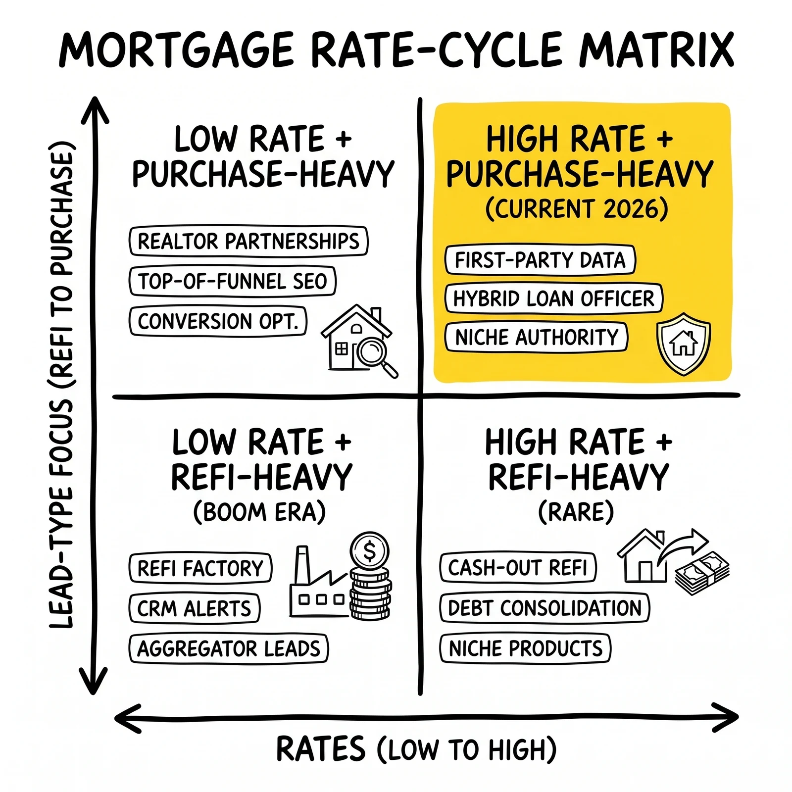
Pricing Strategy Across Rate Cycle Phases
Effective mortgage lead pricing requires a framework that anticipates cycle transitions rather than just reacting to current conditions.
Phase Identification: Where Are We in the Cycle?
Four primary rate cycle phases require different pricing approaches:
Phase 1: Rates Rising Rapidly
- Refinance volume contracting, purchase holding
- CPL for refinance rising (scarcity) or buyer exit (economics fail)
- Home equity CPL increasing as demand builds
- Buyer count decreasing, concentrating revenue among fewer relationships
Phase 2: Rates Elevated and Stable
- Refinance market thin, operating on a small eligible pool
- Purchase demand normalized at lower volume
- Home equity demand mature and stable
- Pricing at equilibrium for current conditions
Phase 3: Rates Beginning to Fall
- Refinance demand beginning to build from recent high-rate vintage borrowers
- Volume recovery lag of 4-8 weeks behind rate movement
- Competition increasing as buyers sense opportunity
- First-mover advantage in securing capacity before CPL rises
Phase 4: Rates Falling Rapidly
- Refinance volume surging, potentially overwhelming buyer capacity
- CPL compression as supply outpaces buyer processing capacity
- Purchase volume recovering but lagging
- Margin squeeze at seller level despite high volume
Phase-Specific Pricing Tactics
In Phase 1 (Rising Rates):
Lock in buyer agreements before CPL rises. Buyers who are still active in the market have not yet repriced upward – they are operating on last month’s cost assumptions. Negotiate volume agreements at current pricing with 60-90 day terms. When volume contracts further and CPL rises, your existing agreements protect margins.
Shift product mix toward home equity where CPL is rising with demand. This is not simply chasing a trend – home equity economics genuinely improve in rising rate environments.
Reduce fixed cost commitments. Platform contracts, staffing levels, and media commitments sized for peak refinance volume become expensive overhead when volume contracts. Convert fixed costs to variable where possible.
In Phase 2 (Elevated, Stable):
Optimize for current conditions rather than waiting for change. Operators who spend Phase 2 holding back capacity in anticipation of rate declines miss revenue that could fund infrastructure for Phase 3 and 4.
Build buyer relationships in adjacent segments. Credit unions, community banks, and specialty lenders are more active in elevated rate environments. Developing these relationships during Phase 2 provides diversity that improves Phase 3 responsiveness.
Invest in conversion optimization. When volume is constrained, squeezing more conversions from existing lead flow improves economics without requiring rate change.
In Phase 3 (Beginning to Fall):
This is the highest-value phase for operators who are positioned. The window between “rates clearly moving lower” and “buyers fully repriced their CPL upward” typically runs 3-6 weeks.
Tactics for Phase 3:
- Pre-negotiate CPL increases with key buyers before market awareness catches up
- Reactivate dormant refinance landing pages and traffic sources before competitors
- Contact dormant buyer relationships – brokers and lenders who exited the market in Phase 1
- Increase media spend in refinance keywords before CPL inflation in the ad auction
In Phase 4 (Rapidly Falling):
Volume surges can overwhelm operations that are not prepared. Infrastructure constraints – call center capacity, CRM processing speed, validation API rate limits – can create bottlenecks that reduce effective lead quality despite high raw volume.
CPL compression is the primary pricing challenge. As lead supply increases faster than buyer capacity, the auction clears at lower prices. Operators who locked in favorable pricing in Phase 3 maintain margin; those selling spot market deal with compressed CPL.
Buyer return rates can spike during volume surges because quality processes get skipped in the rush. Maintain validation and quality standards even under volume pressure – return credits from poor quality leads erode Phase 4 revenue.
Setting CPL Floors Across the Cycle
CPL floors protect operators from agreeing to pricing that does not cover costs. Floors should be calculated based on variable cost structure plus required margin, not based on what buyers offer:
CPL Floor Components:
- Traffic acquisition cost per lead (varies by channel and rate environment)
- Validation and verification cost per lead ($0.50-3.00 depending on stack)
- Platform and infrastructure cost per lead (fixed cost divided by volume)
- Return credit reserve (historical return rate × average CPL)
- Required margin contribution
In Phase 1, variable traffic acquisition costs for refinance leads increase because auction competition intensifies for the smaller eligible audience. CPL floors must reflect these higher acquisition costs.
In Phase 4, high volume compresses traffic acquisition CPL, allowing lower CPL floors – but also creating pressure from buyers who observe the market movement and push harder on price negotiations.
The Float Problem in Rate Volatile Markets
The mortgage lead business’s cash flow structure creates specific risk during rate volatility. Operators typically pay traffic acquisition costs within 15-30 days of accrual but collect from lead buyers on 30-60 day terms. This structure creates a working capital float that becomes more expensive during rate transitions.
Volume surge scenario: When refinance volume surges during rate declines (Phase 3-4), operators must fund increased traffic spend immediately but wait 30-60 days to collect from buyers. A $100,000 monthly business that doubles in a week requires $100,000+ in additional working capital to fund the ramp before revenue catches up.
Volume contraction scenario: When volume contracts (Phase 1), buyer payment terms that were generous in stable conditions become a concentration of outstanding receivables. Operators with 60-day terms have two months of receivables from buyers who may be experiencing their own financial stress.
Risk mitigation approaches:
- Maintain 6-12 months of operating expense reserves for rate transition buffer
- Negotiate shorter payment terms (Net-30 preferred) with new buyers during favorable market conditions
- Establish credit lines that can fund volume surge periods without equity dilution
- Diversify buyer concentration – no single buyer representing more than 25% of revenue reduces both volume risk and payment risk
Frequently Asked Questions
How quickly do mortgage lead CPL changes follow Fed rate announcements?
The full CPL adjustment typically takes 30-90 days from a Fed rate announcement, not days. The 10-year Treasury yield adjusts within days; primary mortgage rates move within a week; lender appetite adjusts within 2-4 weeks; consumer behavior shifts within 4-8 weeks. The earliest visible CPL effect appears in buyer negotiation stances at 2-3 weeks. Full market equilibrium at new pricing takes 60-90 days.
Why do refinance CPL and volume move in opposite directions?
In high-rate environments, qualified refinance candidates are scarce. Buyers compete for a small pool of in-the-money borrowers, pushing CPL up. In low-rate environments, volume is massive but buyers’ capacity to process leads is constrained, pushing CPL down. Volume and CPL are inversely correlated for refinance because supply and demand dynamics work differently than in most markets – more total leads does not mean more qualified leads, it means more buyers competing for similar qualified volume.
What rate level triggers meaningful refinance volume recovery?
As of 2025-2026, the largest pool of potential refinancers consists of homeowners who financed at 2022-2024 peak rates (6.5-7.5%). Rates would need to fall approximately 75-100 basis points below their existing rate to trigger meaningful inquiry volume from this cohort. Separately, rates falling below 5.5% would begin activating some demand from the larger pool of pre-2022 homeowners, though most with sub-4% rates would need rates below 4.5% for the math to work.
How should buyer agreements be structured during rate uncertainty?
Shorter contract terms with volume flexibility outperform long fixed-term agreements during rate volatility. Monthly pricing agreements allow both parties to adjust as market conditions change. Volume caps protect buyers who cannot absorb unlimited leads at a fixed price. Volume minimums protect operators who need predictable revenue to justify marketing investment. The optimal structure: monthly CPL with 30-day notice for changes, volume bands with pricing tiers for over-delivery, and 60-day termination with wind-down provisions for either party.
Which lender types provide the most stable lead buying through rate cycles?
Credit unions and community banks provide the most stable purchasing across rate cycles because they have lower margin requirements and longer-term relationship orientation. Large national lenders provide the highest peak purchasing capacity but the most volatile behavior across cycles. Independent brokers are the most responsive to current market conditions but also the most volatile – they can ramp quickly but also exit quickly. A diversified buyer network with representation across all three types provides more stable revenue than concentration in any single lender category.
Sources
- Mortgage Bankers Association Weekly Application Survey – MBA.org
- Federal Housing Finance Agency House Price Index – FHFA.gov
- Freddie Mac Primary Mortgage Market Survey (weekly rate data) – FreddieMac.com
- LendingTree Q2 2025 Financial Results and Segment Revenue Data – Investor.LendingTree.com
- Federal Reserve Board: Federal Open Market Committee meeting minutes and economic projections – FederalReserve.gov
- Consumer Financial Protection Bureau: TRID and RESPA enforcement actions – CFPB.gov
- NMLS Consumer Access licensing database – NMLSConsumerAccess.org