A comprehensive framework for growing lead operations from 1,000 to 100,000 monthly leads while maintaining the quality metrics that keep buyers happy and margins intact.
You doubled your lead volume last quarter. Your revenue grew 87%. Your buyers started complaining, then pausing their accounts, then canceling contracts entirely. By the time you understood what happened, you’d lost three of your top five buyers and spent $400,000 acquiring leads that nobody would purchase.
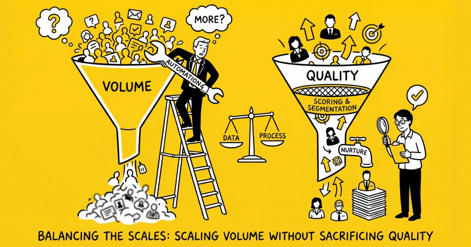
This is the scaling trap, and it destroys more lead generation businesses than any other single factor.
The fundamental tension is real: every mechanism that increases lead volume tends to degrade lead quality. Algorithms find cheaper traffic to fulfill larger budgets. Broader targeting reaches less qualified audiences. Faster growth outpaces quality control infrastructure. Those who navigate this tension successfully don’t eliminate it – they manage it systematically.
This guide provides the complete framework for scaling lead volume while protecting quality. Not the simplified version where you just “maintain standards.” The operational reality where every scaling decision involves trade-offs, where quality metrics must be defined precisely, and where the difference between success and failure often comes down to whether you built the right systems before you needed them.
Why Quality Degrades During Scaling
Quality degradation during scaling is not random failure. It follows predictable patterns with identifiable causes. Understanding these mechanisms is the first step toward preventing them.
The Three Laws of Scaling Degradation
Law 1: Algorithms Optimize for Cost, Not Quality
When you increase advertising budget, platforms face a choice: find more of the same high-quality conversions, or find cheaper conversions to hit volume targets. The algorithm almost always chooses the latter.
At $500 daily spend, your campaign targets your ideal demographic with precision. At $2,000 daily, the platform exhausts that core audience within hours and expands to secondary segments you never explicitly approved. Google’s Performance Max and Meta’s Advantage+ campaigns accelerate this problem – AI-driven campaign types designed to find conversions wherever they exist, with “wherever” often meaning audiences you would have explicitly excluded given the choice.
The data confirms this pattern. Industry research shows that campaigns scaling beyond 2x original spend without quality controls typically see contact rates drop 15-25% and conversion rates decline 20-30%. These are not outliers – they are the predictable result of algorithmic optimization without quality constraints.
Law 2: Capacity Constraints Create Bottlenecks
Scaling lead generation requires scaling every component of the operation simultaneously. When one component fails to scale, quality suffers.
Consider the cascade: You increase ad spend 50%. Lead volume increases proportionally. But your validation infrastructure still processes the same number of leads per minute, creating queues. Delayed validation means leads arrive to buyers later. Later arrival means lower contact rates. Lower contact rates mean higher return rates. Higher return rates mean buyer complaints. Buyer complaints mean paused accounts. Paused accounts mean unsold inventory. Unsold inventory means revenue collapse.
The bottleneck might be validation speed, buyer capacity, sales team bandwidth, or simple cash flow constraints. The specific failure point varies, but the principle remains: scaling reveals the weakest link in your operation, and that weak link manifests as quality degradation.
Law 3: Measurement Lags Reality
The most dangerous aspect of scaling is the delay between quality degradation and detection. You know your cost per lead on the day of acquisition. You might know contact rates within a week. Conversion rates often take 2-4 weeks. Return patterns stabilize over 30-60 days. Customer lifetime value becomes clear over months or years.
This means aggressive scaling can appear successful for weeks while actually destroying long-term profitability. An operator who doubles spend in January might not fully understand the quality impact until March – by which time they’ve spent another $200,000 acquiring leads of unknown quality.
The 2024-2025 data makes this stark: Google Ads average cost per lead rose to $70.11, up 5% year-over-year. Facebook lead ad CPL increased 20% to approximately $27.66. These platform-wide increases reflect the cumulative effect of advertisers discovering that what looked like efficient scale was actually quality dilution.
Quality Degradation by Traffic Source
Different traffic sources exhibit different degradation patterns during scaling, and understanding these patterns helps you anticipate problems before they materialize.
Paid search through Google and Microsoft represents the highest-intent traffic with the steepest degradation curve. Search audiences are finite – there are only so many people searching “auto insurance quotes” on any given day. Scaling exhausts high-intent keywords first, forcing expansion into broader terms with lower purchase intent. A campaign running profitably on exact match “car insurance quote” gets pushed into broad match “insurance” territory, capturing informational queries alongside purchase intent.
Social media platforms like Meta and TikTok show moderate intent with audience exhaustion as the primary degradation mechanism. These platforms show your ads to the most likely converters first. Scale forces reaching deeper into your target audience, then expanding the audience itself. Frequency metrics creep upward as you exhaust fresh audiences. The same people see your ad five, ten, fifteen times – and your quality score reflects those who converted on exposure twelve rather than exposure one.
Native advertising through Taboola and Outbrain starts with lower baseline quality but shows more gradual degradation. Native advertising audiences are inherently less targeted, so the delta between core and expanded audiences is smaller. However, publisher quality varies dramatically. Scaling often means accessing lower-tier publisher inventory where engagement patterns differ substantially.
Programmatic display remains highly variable, with quality depending entirely on implementation. Programmatic can maintain quality at scale if targeting constraints are properly configured – and collapse immediately if opened for “optimization.”
Defining Quality: Metrics That Actually Matter
Before scaling, you must define exactly what “quality” means for your operation. Vague commitments to “maintain standards” fail because they provide no mechanism for detection or enforcement.
Tier 1: Leading Indicators (Daily Monitoring)
These metrics provide early warning of quality degradation, often before buyers notice problems.
Form Completion Rate
Form completion rate measures visitors who complete a form divided by visitors who start it. This metric matters because declining completion rates often precede quality problems. Lower-quality traffic sources show different form engagement patterns – more abandonment, longer completion times, more field corrections. Maintain this rate within 10% of baseline; a 15% decline demands investigation.
Validation Pass Rate
Validation pass rate tracks leads passing phone, email, and address validation against total leads captured. This is your first objective quality measure. If validation rates drop, you’re capturing more invalid data – regardless of whether it came from fraud, poor-quality traffic, or form usability problems. Industry standard runs 85-95% pass rate for phone validation and 90-98% for email. Track against your own baseline and investigate drops exceeding 5 percentage points.
Duplicate Rate
Duplicate rate measures leads matching existing database records against total leads captured. Scaling often means reaching the same consumers through different channels. Rising duplicate rates indicate audience overlap – you’re paying twice for the same prospects. Typical rates run 5-15% depending on vertical; investigate increases of 3 or more percentage points.
Cost Per Lead (CPL)
Cost per lead divides total advertising spend by leads captured. CPL is necessary but insufficient as a quality indicator. A rising CPL during scaling is expected. A rising CPL with declining quality is catastrophic. Accept 15-30% CPL increase during controlled scaling phases, but investigate increases beyond budget projections.
Tier 2: Quality Indicators (Weekly Monitoring)
These metrics reveal quality issues before they become crises, typically with a 3-7 day lag.
Contact Rate
Contact rate measures leads successfully contacted divided by total leads delivered to buyers. This is the first buyer-side quality metric, measuring whether your leads actually answer when called – the fundamental requirement for conversion. Fresh leads typically show 40-60% contact rates while aged leads at 48 hours or more drop to 20-40%. Vertical variations are substantial: auto insurance averages 45-55%, solar runs 20-35%, and legal personal injury shows 15-25%. Maintain within 10% of buyer baseline; a 15% decline typically triggers buyer concern.
Return Rate
Return rate tracks leads returned by buyers against total leads sold. Returns directly attack profitability. A 5-point increase in return rate can transform a profitable operation into a loss-maker. Industry average runs 8-15%, with well-managed operations targeting under 10%. Rates above 15% strain buyer relationships. Set your threshold at maximum 5-point increase from baseline before intervention.
Qualification Rate
Qualification rate measures leads qualifying for a buyer’s product against leads contacted. This reveals whether your leads match buyer criteria when conversations actually happen. A lead that answers but can’t afford the product or doesn’t meet eligibility requirements wastes buyer resources. Maintain within 15% of buyer baseline.
Tier 3: Conversion Indicators (Monthly Monitoring)
These metrics reveal the ultimate quality picture but arrive too late for course correction.
Lead-to-Sale Conversion Rate
Lead-to-sale conversion rate divides customers acquired by leads delivered. This is what buyers ultimately care about. Conversion rates determine whether leads are profitable for buyers – and whether buyers will continue purchasing. Benchmarks vary by vertical: auto insurance runs 4-7%, mortgage 1-2%, solar 1-3%, and legal personal injury 0.5-1%. Maintain within 80% of buyer baseline; significant decline triggers contract renegotiation or termination.
Revenue Per Lead (RPL)
Revenue per lead divides total revenue collected by total leads delivered. RPL accounts for returns, price adjustments, and payment failures. It’s your actual economic outcome, not your theoretical one. Maintain within 85% of baseline.
Buyer Satisfaction Score
Buyer satisfaction score provides qualitative assessment from buyer communications. Numbers don’t capture everything. A buyer who makes excuses to avoid calls is sending a signal. A buyer who proactively requests volume increases is sending the opposite signal. Watch for any negative trending.
The Quality-Volume Framework
Sustainable scaling requires a systematic framework that integrates quality monitoring into every growth decision. This framework provides the structure.
Phase 1: Foundation (Before Scaling)
No scaling should begin until foundation elements are in place.
Document Baseline Metrics
Capture 30-60 days of stable-state metrics for every quality indicator. Record averages, standard deviations, day-of-week patterns, and traffic source breakdowns. This baseline becomes your comparison point for all scaling decisions.
Without documented baselines, you cannot objectively identify quality degradation. You’ll rely on buyer complaints – which arrive too late for intervention.
Build Buyer Capacity
The most common scaling failure has nothing to do with traffic quality. It occurs when operators scale lead volume beyond buyer capacity, forcing sales to secondary buyers at discounted rates or warehousing leads until they age out of value.
Before increasing ad spend, confirm in writing that your primary buyer can absorb increased volume with specific numbers, that secondary buyers exist for overflow with minimum two under contract, and that your float capacity supports the increase. Calculate required capital as new daily spend multiplied by 45-60 days.
Establish Quality Infrastructure
Validation systems must scale before lead volume scales. If your current infrastructure processes 1,000 leads daily at 99.5% accuracy, can it handle 3,000 daily at the same accuracy? Or will processing delays create queues that degrade freshness?
Key infrastructure requirements include real-time validation with sub-second response times, fraud detection across multiple signal types including IP, device, and behavior, duplicate checking against current and historical databases, and consent verification with documentation systems. Budget $0.30-$0.50 per lead for comprehensive validation – costs that prevent vastly larger losses from bad leads.
Phase 2: Controlled Acceleration
With foundations in place, scaling proceeds through measured increments with continuous monitoring.
The 15-20% Weekly Protocol
Increase spend by 15-20% weekly, measure quality for 5-7 days, and proceed only if thresholds hold. This pace allows algorithm stabilization, quality monitoring, and buyer feedback loops to function.
The increment matters more than intuition suggests. Scaling too slowly at 5-10% takes 4-6 months to double spend, and market conditions change before you scale. The optimal 15-20% range doubles spend in 6-8 weeks while providing time to catch degradation before compounding. Scaling too fast at 30% or more causes quality degradation to outpace measurement capability, with problems compounding before detection.
Source Diversification Protocol
Single-source scaling hits diminishing returns faster than diversified scaling. Rather than pushing one platform from $20K to $80K monthly, scale across multiple sources:
| Phase | Microsoft | Native | Total | ||
|---|---|---|---|---|---|
| Start | $20K | - | - | - | $20K |
| Phase 1 | $28K | $7K | - | - | $35K |
| Phase 2 | $36K | $12K | $7K | - | $55K |
| Phase 3 | $45K | $18K | $12K | $5K | $80K |
This approach caps individual source scaling at 60% during any phase while achieving 4x overall growth. Target allocation for sustainable scaling places 60% on your primary, proven source, 30% on secondary sources with established quality, and 10% on testing new sources.
The 72-Hour Stabilization Rule
After any budget increase, allow 72 hours for platform algorithms to stabilize. Day-one performance after a budget change is not representative. Algorithms require 48-72 hours to optimize delivery patterns around new budget levels.
In practice, a Monday budget increase should not be evaluated until Thursday at the earliest. Friday budget changes will produce distorted results through the weekend. Platform updates require additional stabilization time beyond the standard window.
Phase 3: Quality-Constrained Optimization
Once you reach target volume, focus shifts from growth to optimization within quality constraints.
Quality Floor Enforcement
Define absolute quality floors that cannot be crossed regardless of volume goals. Contact rate should never fall below 80% of buyer baseline. Return rate should never exceed baseline plus 5 percentage points. Conversion rate should never drop below 75% of buyer baseline. When any floor is approached, pause scaling and diagnose before proceeding.
Source-Level Quality Management
Not all leads are created equal, and not all sources produce equal quality. Track quality metrics by source and enforce source-specific standards.
A source delivering leads at $30 CPL with 5% return rate is more valuable than a source at $25 CPL with 15% return rate. Consider the math:
| Metric | Source A | Source B |
|---|---|---|
| CPL | $30 | $25 |
| Sale Price | $50 | $50 |
| Return Rate | 5% | 15% |
| Net Revenue/Lead | $47.50 | $42.50 |
| Gross Margin | $17.50 | $17.50 |
| Return Cost | -$1.50 | -$3.75 |
| Actual Margin | $16.00 | $13.75 |
Source A produces 16% higher actual margin despite 20% higher CPL. Quality-adjusted source management reveals true economics.
Buyer Communication Protocol
Proactive communication prevents relationship damage during scaling. When beginning a scale phase, inform buyers: “We are increasing volume over the next 8 weeks. We anticipate slight quality normalization as we expand sources. Our target is to maintain contact rates above X%. We will check in weekly with updates.”
This sets expectations, demonstrates professionalism, and creates space for adjustment without surprise.
The Volume-Quality Trade-off Curve
The relationship between volume and quality follows a curve with predictable phases. Understanding where you sit on this curve informs every scaling decision.
The Free Zone (0-50% Increase)
During initial scaling, quality often holds steady or improves slightly. The platform finds more of your existing audience at similar efficiency. Typical metrics show CPL increasing 5-15%, contact rate stable or declining slightly by 1-3%, conversion rate stable, and return rate stable.
This phase creates dangerous confidence. Operators assume quality will remain stable at any scale – an assumption that fails spectacularly in later phases.
The Friction Zone (50-150% Increase)
Quality begins degrading measurably in this phase. Platforms exhaust core audiences and expand into secondary segments. CPL increases accelerate. Contact and conversion rates show consistent decline. Typical metrics show CPL increasing 20-40%, contact rate declining 8-15%, conversion rate declining 10-20%, and return rate increasing 3-8 percentage points.
This is where most practitioners fail. They see volume increasing, accept the CPL hit as “cost of growth,” and miss downstream quality degradation until buyers complain.
The Cliff (150%+ Increase)
Quality collapses at this stage. Platforms rely heavily on low-quality inventory, expanded audiences, and non-core placements. Even if CPL stabilizes – platforms often find cheap conversions at scale – leads generate minimal value. Typical metrics show CPL highly variable and sometimes decreasing as quality craters, contact rate declining 20-35%, conversion rate declining 30-50%, and return rate reaching 20-30% or higher, putting buyer relationships at risk.
Recovery from this phase requires significant pullback, often returning to baseline spend levels and rebuilding.
Identifying Your Position
Your position on the curve depends on several factors. Vertical matters: insurance leads have higher tolerance for volume scaling than legal leads, and home services scale more predictably than mortgage during rate volatility. Traffic source affects the curve shape: Google Search has a steeper curve than Facebook because search intent is more targeted initially, while display and native have flatter curves with quality varying more at any spend level. Geographic concentration plays a role since operations targeting a single state hit audience saturation faster than national campaigns. Buyer thresholds also matter: a buyer requiring 70% contact rates has less tolerance for degradation than one operating at 50% baseline.
When to Pause Scaling
Knowing when to stop is more valuable than knowing how to accelerate. Certain signals require immediate scaling pause.
Hard Stop Signals
Buyer communication signals demand immediate attention. When a buyer requests volume reduction, mentions quality concerns unprompted, delays payment (which may indicate cash flow stress from conversion issues), or when return rates exceed contractual thresholds – these all require you to stop scaling immediately.
Data signals are equally important. Contact rate dropping more than 15% week-over-week, return rate increasing more than 5 percentage points week-over-week, CPL exceeding profitability threshold at current buyer pricing, or three or more quality metrics simultaneously approaching thresholds all warrant a pause.
Market signals also matter. Seasonal demand decline such as insurance Q4 slowdown or mortgage during rate spikes, major regulatory changes affecting your vertical, or competitive intensity spikes during political advertising seasons or open enrollment periods all call for caution.
The 48-Hour Rule
When concerning signals appear, allow 48 hours before major decisions. Quality metrics are inherently noisy. What looks like degradation Monday may resolve Wednesday as algorithms stabilize.
The exception to this rule involves buyer communication requesting changes, which requires immediate response regardless of data patterns. The relationship matters more than your analysis timeline.
Recovery Protocol
When quality degradation requires pullback, follow a specific sequence. Reduce spend 30-40% immediately – not incrementally. Return to a spend level where quality was previously stable. Then isolate degradation sources by reviewing source-level quality data during the degradation period. Communicate with buyers proactively, explaining the situation and your response. Pause underperforming sources entirely rather than reducing budgets. Finally, restart the 15-20% weekly protocol once stability returns.
Remember that the audience available at $50K monthly is fundamentally different from the audience at $25K monthly. You cannot simply “reduce spend” and expect the same quality you achieved before scaling.
Infrastructure for Quality at Scale
Scaling without infrastructure is like driving faster without better brakes. The systems that worked at 1,000 leads monthly will fail at 10,000.
Real-Time Validation Architecture
Every lead must pass through validation before acceptance, with results in milliseconds rather than minutes.
Phone validation must include line type detection for mobile, landline, and VoIP, carrier lookup for deliverability signals, DNC registry checking against federal and state lists, disconnected number detection, and reassigned number database checking.
Email validation must include syntax verification, domain existence and MX record confirmation, disposable email detection, and deliverability testing via SMTP verification.
Address validation must include CASS certification for mailing addresses, geocoding for property verification, and property data append where relevant such as homeownership and home value.
Budget $0.05-$0.25 per lead for validation services. At scale, negotiate volume pricing.
Fraud Detection Systems
Approximately 30% of third-party leads contain fraudulent or materially false information. This is not a minor quality issue – it’s a structural feature of the lead economy requiring systematic defense.
IP and device analysis should cover geographic consistency between IP location and stated address, proxy and VPN and Tor detection, IP reputation scoring from aggregated intelligence, and device fingerprinting for repeat submission detection.
Behavioral analysis should examine time-on-page since impossibly fast completion indicates automation, mouse movement and click pattern analysis, typing dynamics to distinguish humans from bots, and form field progression patterns.
Velocity checking should track submissions per IP per time window, submissions per device per time window, and submissions per phone or email per time window.
Budget $0.02-$0.10 per lead for fraud detection services. Comprehensive prevention costs far less than fraud losses.
Quality Scoring Models
Beyond pass/fail validation, quality scoring predicts downstream performance for individual leads.
Input variables include traffic source and campaign, form completion time and patterns, geographic and demographic attributes, time of day and day of week, device and browser characteristics, and validation results with confidence levels.
Scoring output provides probability of contact, probability of qualification, probability of conversion, and predicted lifetime value tier.
Applications include real-time routing to appropriate buyers based on predicted quality, dynamic pricing based on quality tier, and source optimization based on quality-adjusted ROI.
Sophisticated quality scoring requires data science expertise or specialized platforms. The investment becomes worthwhile at scale where marginal improvements produce substantial dollar impact.
Buyer Feedback Loops
Quality tracking depends on buyer data. Build systematic feedback loops with different cadences. Daily feedback should include delivery confirmations and return notifications. Weekly feedback should cover contact and qualification rate reports. Monthly feedback should provide conversion and revenue-per-lead analysis. Quarterly feedback should involve relationship reviews and goal alignment.
Those who scale successfully receive buyer feedback in days rather than weeks. This feedback velocity determines how quickly you can detect and respond to quality issues.
Case Study: Scaling from 2,500 to 25,000 Monthly Leads
This case study follows a home services lead generation operation through 12 months of controlled scaling.
Starting Position
At Month 0, the operation generated 2,500 monthly leads at $87,500 monthly ad spend, averaging $35 CPL. Traffic came entirely from Google Ads, flowing to a single primary buyer – a regional HVAC and plumbing company. Contact rate stood at 58%, return rate at 8%, lead-to-sale conversion at 9%, and revenue per lead at $48 after returns.
Phase 1: Foundation Building (Months 1-2)
The team documented baseline metrics across all quality indicators and contracted two secondary buyers at 15-20% lower pricing. They tested Facebook Ads with $5,000 spend, achieving $28 CPL and 52% contact rate. They upgraded validation infrastructure for sub-second processing and built a daily quality dashboard with source-level tracking.
By Month 2 end, monthly spend reached $100,000 split between Google at $87,500 and Facebook at $12,500. Monthly leads grew to 3,200 while contact rate held at 57% within baseline and return rate stayed at 8.5% within baseline.
Phase 2: Controlled Scaling (Months 3-6)
The approach followed 15% weekly spend increases with strict quality monitoring.
In Month 3, a Google CPL spike of 28% week-over-week triggered investigation. Performance Max had expanded to mobile app placements. Excluding that inventory returned CPL to acceptable range within one week.
Month 4 brought Microsoft Ads expansion at $8,000 monthly, achieving $32 CPL and 61% contact rate – higher quality than Google average at this scale.
Month 5 revealed buyer capacity constraints. The primary buyer reached 3,500 monthly lead capacity, requiring secondary buyer activation for overflow at 18% lower pricing.
Month 6 required Facebook adjustment. Contact rate declined to 48%, prompting tightened audience targeting. This reduced volume but improved quality, with incremental budget shifting to Microsoft.
By Month 6 end, monthly spend reached $175,000 allocated across Google at $115,000, Facebook at $28,000, and Microsoft at $32,000. Monthly leads hit 6,800. Contact rate showed 55%, down 5% from baseline and monitored closely. Return rate ran 10%, up 2 points from baseline but within threshold.
Phase 3: Diversification (Months 7-9)
The approach added native advertising while holding search and social spend stable.
Month 7 launched Taboola with $15,000 test budget. CPL came in at $22 but contact rate showed only 41%. Pausing underperforming publishers improved contact rate to 49%.
Month 8 brought good news: the primary buyer requested volume increase after internal expansion, raising capacity to 5,500 leads monthly. Google scaling resumed at 10% weekly.
Month 9 added Outbrain at $12,000 monthly, with performance similar to Taboola after publisher optimization.
By Month 9 end, monthly spend reached $260,000: Google at $155,000, Facebook at $35,000, Microsoft at $42,000, and native at $28,000. Monthly leads hit 12,400. Contact rate showed 53%, down 9% from original baseline with buyers informed. Return rate held at 11.5% within acceptable range.
Phase 4: Optimization (Months 10-12)
The approach shifted focus to quality improvement rather than further volume growth.
Month 10 implemented AI-based quality scoring, routing highest-quality leads to the primary buyer and medium-quality to secondary buyers. Primary buyer contact rate improved to 59% despite overall rate decline.
Month 11 introduced three-tier pricing based on quality scores: premium leads at $55, standard at $45, and economy at $35. This increased blended revenue per lead despite increased secondary buyer share.
Month 12 fine-tuned source allocation based on quality-adjusted ROI. Facebook spend decreased where quality lagged. Microsoft and native spend increased where quality-adjusted returns exceeded targets.
Final Month 12 results showed monthly spend at $310,000 and monthly leads at 24,800 – approximately 10x starting volume. Blended CPL came in at $12.50. Source mix showed Google at 48%, Microsoft at 18%, native at 19%, and Facebook at 15%. Contact rate ran 52% overall but 62% for the primary buyer tier. Return rate held at 12%. Revenue per lead reached $44 after returns and tier mix. Buyer count grew to 5, with one primary and four secondary.
Key Lessons
Foundation came first. Two months of preparation prevented problems that would have derailed scaling later.
Diversification preserved quality. No single source exceeded 50% of spend, limiting exposure to any platform’s degradation patterns.
Weekly monitoring caught problems early. Month 3’s placement issue and Month 6’s Facebook quality decline were resolved before buyer impact.
Buyer capacity required parallel development. Five buyers were necessary to absorb 25,000 monthly leads. This capacity required relationship building throughout the scaling period.
Quality-based routing protected relationships. The primary buyer received highest-quality leads, maintaining relationship strength despite overall quality normalization.
Timeline was 12 months, not 12 weeks. Patient scaling created sustainable 10x growth. Aggressive compression would have destroyed buyer relationships.
Frequently Asked Questions
What is the optimal rate for scaling lead generation volume?
The optimal scaling rate is 15-20% weekly budget increases with 5-7 days of quality monitoring between increments. This pace doubles volume in 6-8 weeks while maintaining visibility into quality degradation. Faster scaling at 30% or more weekly consistently produces quality problems that damage buyer relationships before detection. Slower scaling under 10% weekly may miss market opportunities but rarely causes quality issues. The 15-20% range balances growth velocity against quality monitoring capability.
How do I know if quality degradation is temporary algorithm noise or a real problem?
Apply two rules: the 72-hour rule and the two-period rule. First, wait at least 72 hours after any budget change before evaluating quality metrics – platforms need this time for algorithmic stabilization. Second, require two consecutive measurement periods showing decline before treating it as a real problem. Single-period fluctuations are often noise; consecutive-period declines indicate systematic issues requiring intervention.
My dashboard metrics look fine but my buyer says quality is declining. Who is right?
Your buyer is right. Always. Buyers experience quality through their sales team’s daily reality – calls that don’t connect, conversations that reveal unqualified prospects, deals that fall through. If their experience diverges from your metrics, your metrics are measuring the wrong things or measuring at the wrong granularity. Align your tracking to buyer experience rather than defending your dashboard.
What percentage quality decline is acceptable during scaling?
Most operations can sustain 10-15% decline in contact and conversion rates while remaining profitable. Beyond 15%, profitability erodes quickly and buyer relationships strain. Set thresholds at 85-90% of baseline metrics, giving room for normal scaling friction while preventing serious degradation. Communicate expected quality normalization to buyers before scaling begins.
Should I scale vertically on one platform or diversify across multiple platforms?
Diversify. Single-platform scaling hits diminishing returns faster because you exhaust quality inventory on that platform. Four sources at $25K each typically produce higher average quality than one source at $100K. Target no more than 50-60% of spend on any single platform during active scaling. Diversification also protects against platform-specific risks like account suspensions or policy changes.
How do I handle buyer capacity constraints when generating more leads than buyers can absorb?
Build secondary and tertiary buyer relationships before hitting capacity constraints – not after. Secondary buyers typically pay 15-30% less, which changes unit economics but maintains revenue. The worst outcome is generating leads you cannot sell; warehoused leads lose 50% or more of value within 48 hours for most verticals. Develop buyer relationships during stable periods by testing 50-100 leads with new buyers quarterly.
What infrastructure investments should I make before scaling?
Three categories require investment before scaling. Validation speed must deliver sub-second processing with no queuing at target volume. Fraud detection needs multi-signal analysis covering IP, device, and behavior. Quality tracking requires source-level metrics with daily granularity. Budget $0.30-$0.50 per lead for validation and fraud prevention, plus $2,000-$10,000 monthly for tracking infrastructure depending on volume. These investments prevent far larger losses from quality problems.
How long does it typically take to scale from 5,000 to 50,000 monthly leads?
Plan for 9-12 months minimum for sustainable 10x scaling. The 15-20% weekly protocol doubles volume every 6-8 weeks, but foundation building, buyer development, and periodic consolidation phases extend the timeline. Attempts to compress this timeline – common when operators have capital to deploy – consistently produce quality collapses that force pullbacks. Patient scaling builds sustainable operations; aggressive scaling builds case studies in failure.
What metrics should I share with buyers during scaling?
Share contact rate trends, return rate trends, and any quality initiatives you’re implementing. Do not share CPL, margin, or source-level details that reveal your economics. Frame communication around quality maintenance: “We’ve scaled volume 40% while maintaining contact rates within 8% of baseline.” Proactive transparency builds trust; reactive explanation after problems damages it.
How do I recover if I’ve already scaled too fast and quality has degraded?
First, reduce spend 30-40% immediately – not incrementally. Return to a spend level where quality was historically stable. Second, communicate with affected buyers before they contact you. Third, isolate which sources contributed most to degradation and pause the worst performers entirely. Fourth, allow 2-3 weeks for stabilization before restarting controlled scaling using the 15-20% protocol. The audience at reduced spend is different from the audience at peak spend – you’re effectively rebuilding.
Key Takeaways
-
Quality degradation during scaling is predictable, not random. Advertising platforms expand to lower-quality inventory as budgets increase. The 15-20% weekly scaling protocol provides visibility into degradation before it compounds into buyer relationship damage.
-
Define quality metrics precisely before scaling begins. Vague commitments to “maintain standards” fail because they provide no mechanism for detection or enforcement. Establish baselines, set thresholds, and track daily.
-
Diversification beats concentration. Four traffic sources at $25K each produce higher average quality than one source at $100K. No single platform should exceed 50% of total spend during active scaling.
-
Buyer capacity must scale before lead volume. The constraint on most operations is not traffic availability – it is buyer absorption capacity. Build relationships during stable periods so capacity exists when scaling creates demand.
-
Infrastructure investment precedes scaling. Validation systems, fraud detection, and quality tracking must handle target volume before you attempt to reach it. Scaling reveals the weakest link in your operation.
-
Twelve months beats twelve weeks. Sustainable 10x scaling typically requires 9-12 months of disciplined execution. Compressed timelines produce quality collapses that force pullbacks and damage buyer relationships.
-
Your buyer’s experience is the ultimate quality metric. When buyer feedback diverges from your dashboard, your dashboard is wrong. Align measurement to buyer reality, communicate proactively, and treat relationship preservation as a primary objective.
-
Recovery requires significant pullback. If quality has already degraded, reduce spend 30-40% immediately and rebuild from a stable foundation. The audience at reduced spend is different from the audience at peak spend.
The lead economy rewards operators who scale patiently and punishes those who chase volume at the expense of quality. The buyers who pay premium prices for your leads have options. The moment your leads stop converting, those buyers move to competitors who prioritized sustainable quality over impressive growth charts. Scale like your buyer relationships depend on it – because they do.