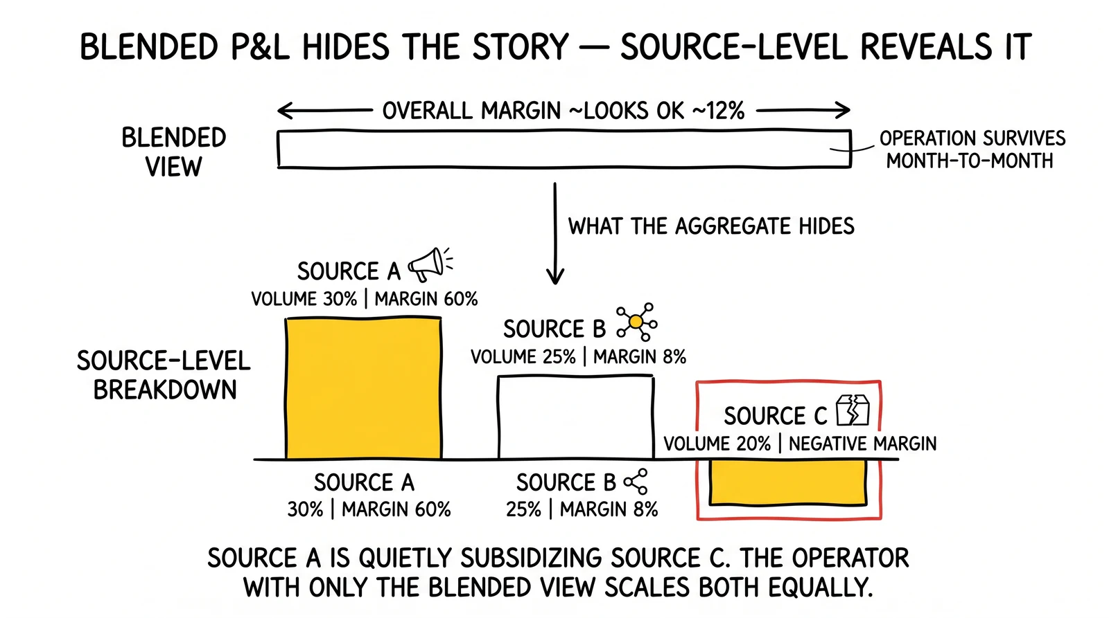
The blended P&L looks acceptable. Revenue covers costs. Margins are thin but present. The operation survives month to month.
The source-level P&L tells a different story. Source A generates 30% of volume and 60% of margin. Source B generates 25% of volume and 8% of margin. Source C generates 20% of volume and negative margin that Source A’s excess is quietly subsidizing.
The operator who sees only the blended view continues treating all three sources equally, scaling the one that is losing money right alongside the one that is building the business. The operator with source-level visibility cuts Source C, renegotiates Source B, and doubles down on Source A. The margin impact compounds quarterly.
This guide builds the P&L model that enables that visibility. The math is not complex. The discipline to collect the data and run it consistently is where most operations fall short.
The Source-Level P&L Framework
A source-level profit model assigns revenue and costs to individual traffic sources rather than aggregating everything into a single operational view. The model has four components: revenue attribution, variable cost attribution, overhead allocation, and net margin calculation.
Revenue Attribution by Source
Revenue attribution answers: for each lead this source generated, what was actually collected?
Gross revenue: The invoice value of leads delivered from this source. For ping-post operations, this is the winning bid price per lead times volume. For fixed-price programs, it is the contracted price times volume.
Return deductions: Leads returned by buyers reduce revenue. Attribution requires matching each return to its originating source. Most distribution platforms track this, but many operators never extract the data at the source level. Pull source-tagged return reports rather than aggregate return data.
Chargeback deductions: Beyond formal returns within the return window, some buyers issue chargebacks for billing disputes. These post-window deductions are less common but material when they occur. Track them separately from returns because they represent a different failure mode – typically a billing process issue rather than a lead quality issue.
Bad debt reserve: Buyers who do not pay leave revenue booked but uncollected. For well-managed buyer relationships with credit limits and payment terms, bad debt runs 1–3% of gross revenue. Operations with looser credit practices can see 5–8% bad debt rates during market downturns when marginal buyers fail. Allocate a bad debt reserve against each source’s revenue proportional to the payment track record of the buyers that source feeds.
Net revenue formula:
Net Revenue (Source A) = Gross Revenue
                        - Returns (Source A leads)
                        - Chargebacks (Source A leads)
                        - Bad Debt Reserve (% of net)
Variable Cost Attribution
Variable costs attach directly to individual leads without allocation decisions. These are the costs that exist because this specific lead was generated.
Media cost: The click cost, impression cost, or CPM that generated this lead. For owned sources (organic, email), media cost is zero but the labor and platform costs that generated the traffic should appear in overhead. For affiliate traffic, the commission paid per lead is the variable media cost.
Per-lead validation fees: Phone verification, email verification, address validation, IP intelligence, and fraud scoring all run per-lead charges. Capture these at the lead level if your validation stack passes through cost data. If not, aggregate the monthly cost and divide by lead volume for an average allocation.
Consent certification cost: TrustedForm and Jornaya charge per certificate. These costs should appear in the source P&L for the source that generated the certified lead.
Distribution platform per-lead fees: Most distribution platforms charge a per-lead routing fee beyond their base subscription. These attach to each delivered lead and belong in variable costs.
Affiliate or publisher commissions beyond base media cost: For CPA-based affiliate programs, the commission is the primary media cost. For programs with tiered commissions, bonuses, or quality adjustments, all commission components belong in variable cost.
The Source P&L Template
The spreadsheet structure that enables source-level analysis:
| Line Item | Source A | Source B | Source C | Total |
|---|---|---|---|---|
| Gross Lead Volume | 5,200 | 4,800 | 3,100 | 13,100 |
| Return Rate | 6% | 14% | 24% | 12.5% |
| Returns (leads) | 312 | 672 | 744 | 1,728 |
| Net Delivered Volume | 4,888 | 4,128 | 2,356 | 11,372 |
| Average Sale Price | $72 | $68 | $65 | – |
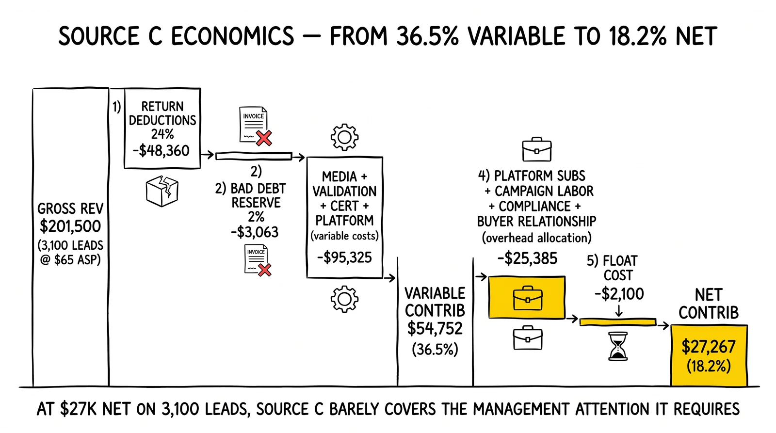
| Gross Revenue | $374,400 | $326,400 | $201,500 | $902,300 |
| Return Deductions | $(22,464) | $(45,696) | $(48,360) | $(116,520) |
| Bad Debt Reserve (2%) | $(7,039) | $(5,614) | $(3,063) | $(15,716) |
| Net Revenue | $344,897 | $275,090 | $150,077 | $770,064 |
| Media / Acquisition Cost | $(104,000) | $(115,200) | $(93,000) | $(312,200) |
| Validation Fees ($0.35/lead) | $(1,820) | $(1,680) | $(1,085) | $(4,585) |
| Certification Costs ($0.25/lead) | $(1,300) | $(1,200) | $(775) | $(3,275) |
| Platform Per-Lead Fees ($0.15/lead) | $(780) | $(720) | $(465) | $(1,965) |
| Variable Contribution | $236,997 | $156,290 | $54,752 | $448,039 |
| Variable Margin % | 68.7% | 56.8% | 36.5% | – |
Before overhead allocation, Source C is already generating 36.5% variable margin – less than half of Source A’s 68.7%. The business case for aggressive Source C reduction or termination is visible without even completing the overhead allocation.
Return and Chargeback Accounting
Returns deserve more careful treatment in source-level P&L than most operators apply. The headline return rate understates the true cost of returned leads by ignoring the processing burden and the opportunity cost.
The True Cost of a Returned Lead
A returned lead costs:
The full acquisition cost of the original lead. Even if the supplier credits back the cost (which many do not, depending on contract terms), there is a timing gap between paying for the lead and receiving the credit.
The return processing labor. Each return requires review against the return policy, verification of the buyer’s claim, credit issuance or dispute filing, and documentation. At 15–25 minutes per return for a modestly complex review process and $25–35/hour fully-loaded labor cost, each return costs $6.25–14.58 in processing. For 500 monthly returns, this is $3,125–7,290 in processing labor that the return rate metric never captures.
The supplier credit recovery delay. If your supplier offers a return credit, there is typically a 30–90 day window to claim it. During that period, you have paid for the lead and not received the credit. The working capital cost of this timing gap is real.
The buyer relationship cost. Elevated return rates from a specific source erode buyer confidence. When buyers see return rates climbing, they reduce bids, lower caps, or exit. The revenue impact of buyer attrition from source quality issues is difficult to quantify at the source level but can be estimated by tracking buyer retention rates alongside source-specific return metrics.
Source-Level Return Reason Analysis
Aggregate return reason data does not identify which sources drive which failure modes. Source-tagged return reason analysis reveals the specific problem to address.
A source generating returns concentrated in “disconnected phone” points to phone verification as the appropriate remediation. A source generating returns concentrated in “qualification mismatch – geographic” points to targeting configuration. A source generating returns concentrated in “consumer denies submitting” points to incentivized or fraudulent traffic. The remediation differs completely depending on the root cause – and the root cause is only visible at the source level.
Chargeback Accounting Mechanics
Chargebacks differ from returns in timing and mechanism. Returns occur within the contracted return window (typically 24–72 hours for real-time leads). Chargebacks occur outside the return window when buyers dispute charges through their payment processor or through a platform dispute process.
For chargeback accounting at the source level:
- Tag every chargeback with the original lead’s source ID at the time of the dispute
- Record the chargeback amount as a negative adjustment against that source’s revenue in the period when the chargeback is settled
- Maintain a trailing 90-day chargeback rate by source to identify sources with post-window quality issues
Chargebacks are rarer than returns but worth tracking separately because they often indicate different quality problems – consent issues, fraud, or systemic misrepresentation – that returns within the window may not surface clearly.
Aging Cost Recognition
Leads that are not sold immediately accumulate aging cost. For lead generation operations that hold inventory (aged leads programs, unsold real-time leads that age to next-day pricing), aging cost represents a real economic drag that source-level models often ignore.
Why Aging Matters in Source P&L
A lead generated at 9am on Monday that does not sell in real-time pricing drops to aged pricing by Tuesday. The acquisition cost is fixed. The revenue decreases as the lead ages. The difference between real-time CPL and aged CPL is the aging cost that the source generated.
For sources with high immediate sell-through rates (90%+ sold within the real-time window), aging cost is minimal. For sources where 20–30% of leads age to next-day or week-old pricing, aging cost is a material margin component.
Calculating Aging Cost by Source
Track for each source:
- Real-time sell-through rate (% sold within first delivery window)
- Average real-time sale price
- Average aged sale price (by aging tier: same-day, next-day, 2–7 day, 7+ day)
- Volume by aging tier
The aging cost per lead from this source equals:
Aging Cost = (Real-time Price - Aged Tier Price) × Volume at That Tier
             divided by Total Volume
A source where 30% of leads age to next-day pricing ($45 average) from real-time pricing ($70 average) incurs an aging cost of $7.50 per lead ($25 price reduction × 30%). This is a source characteristic that the CPL metric never captures but that materially affects contribution margin.
Why Certain Sources Age More
Sources age disproportionately when:
- Traffic is concentrated in low-demand time windows (late night, weekend)
- Consumer intent signals are weaker, reducing buyer bid rates
- Geographic concentration falls outside available buyer coverage
- Qualification failure rates are high, reducing the pool of buyers who will accept the lead
Aging patterns by source identify structural misalignments between traffic timing, consumer intent, and buyer demand that can be addressed through targeting adjustments, routing configuration, or source renegotiation.
Payment Terms Float Allocation
Payment terms create a timing gap that has a real cost. Allocating this cost at the source level requires understanding which buyers purchase which sources’ leads and what payment terms those buyers operate on.
The Float Calculation
For each source, the float cost is:
Monthly Float Cost (Source) = Average Receivables from Source Leads × (Annual Cost of Capital / 12)Receivables from source leads equals the outstanding revenue from that source’s leads that has been invoiced but not yet collected. For a source generating $200,000 monthly in net revenue with 35-day average buyer payment terms, average outstanding receivables are approximately $233,000 (35/30 × $200,000).
At 12% annual cost of capital (cost of the credit line or opportunity cost of tied-up working capital), monthly float cost is $233,000 × (12% / 12) = $2,330, or roughly $0.45 per lead at 5,200 source volume.
Why Float Differs by Source
Sources that feed buyers with slower payment terms incur higher float cost per lead. If Source A predominantly feeds premium buyers who pay on net-15 terms, and Source B feeds newer buyers on net-45 terms, Source A’s float cost is approximately one-third of Source B’s per lead.
This makes payment terms a source-level characteristic worth tracking. When evaluating whether to continue with Source B given its higher float cost, add that cost to its variable costs before comparing contribution margins with Source A.
Float Cost in the Supplier Direction
The float calculation runs both directions. If you pay suppliers before you collect from buyers – the standard pattern in most lead operations – you are financing the gap.
Standard timing in many operations:
- Day 0: Lead generated and delivered
- Day 7–15: Supplier payment due
- Day 30–45: Buyer payment received
The float cost is on roughly 20–30 days of outstanding receivables at any point. Operations running $500,000 monthly at 12% annual capital cost incur approximately $5,000/month in float – about $0.38 per lead at 13,100 monthly volume in the example above. This is real cost that belongs in the P&L model.
Overhead Allocation Methodologies
Overhead costs – platform subscriptions, labor, compliance infrastructure, legal – do not attach to individual leads naturally. They require allocation methodologies that distribute these costs across sources in a way that produces meaningful source-level margins.
The Two Allocation Approaches
Volume-proportional allocation distributes overhead costs based on each source’s share of total lead volume. If Source A generates 40% of leads, it receives 40% of overhead. This approach is simple and defensible for most cost categories.
Revenue-proportional allocation distributes overhead based on each source’s share of net revenue. If Source A generates 45% of revenue despite producing 40% of leads (because its average price is higher), it receives 45% of overhead. Revenue-proportional allocation better represents the causal relationship between source performance and the infrastructure required to support it.
For most operations, the choice between volume and revenue proportion produces similar results unless there are significant price differences between sources. Document the methodology used and apply it consistently – changing methodologies between periods makes trend analysis unreliable.
Overhead Categories and Their Allocation Bases
Platform subscriptions (distribution, CRM, analytics): Volume-proportional. These costs exist to process leads, and volume is the best proxy for processing intensity.
Campaign management labor: Source-proportional based on management time. If a campaign manager spends 40% of their time on Source A campaigns and 20% on Source B, allocate their salary accordingly. For operations where managers work across sources, an estimate based on time logs or reported effort is more accurate than volume proportion.
Compliance infrastructure (legal counsel amortized, compliance staff): Revenue-proportional. Compliance risk scales with revenue, not just volume. A $70 lead carries more regulatory liability than a $25 lead, and the compliance infrastructure cost should reflect that.
Buyer relationship management: Allocate to sources based on which buyers purchase that source’s leads, and in proportion to the effort those buyer relationships require. Sources that feed new, high-maintenance buyers incur more buyer relationship cost than sources feeding established, low-maintenance buyers.
Testing and development costs: These are harder to allocate and are often left at the portfolio level. Testing costs that enable a new source to launch belong to that source once it goes live, amortized over the expected source lifetime. Testing costs for platform improvements that benefit all sources belong at the portfolio level.
The Overhead-Allocated Source P&L
Continuing the earlier example with overhead allocation:
| Line Item | Source A | Source B | Source C | Total |
|---|---|---|---|---|
| Variable Contribution | $236,997 | $156,290 | $54,752 | $448,039 |
| Platform Subscriptions (vol.) | $(7,800) | $(7,200) | $(4,650) | $(19,650) |
| Campaign Labor (by mgmt. time) | $(18,000) | $(14,400) | $(9,600) | $(42,000) |
| Compliance Infrastructure (rev.) | $(14,100) | $(11,245) | $(6,135) | $(31,480) |
| Buyer Relationship Labor | $(6,000) | $(9,000) | $(5,000) | $(20,000) |
| Float Cost (by receiver timing) | $(2,800) | $(3,400) | $(2,100) | $(8,300) |
| Overhead Allocated | $(48,700) | $(45,245) | $(27,485) | $(121,430) |
| Net Contribution | $188,297 | $111,045 | $27,267 | $326,609 |
| Net Margin % | 54.6% | 40.4% | 18.2% | 42.4% |
Source C, which looked manageable at 36.5% variable margin, is generating 18.2% net margin after overhead allocation. The business is cross-subsidizing Source C operations at the expense of Source A’s returns.
The decision framework is now clearer: reduce Source C aggressively, renegotiate terms with suppliers to improve its variable economics, or terminate and redeploy the management attention to Source A expansion.
Marginal vs. Average Cost Analysis
Average cost metrics guide steady-state operations. Marginal cost analysis guides investment decisions – where to put the next dollar of spend.
Why Average and Marginal Cost Diverge
Average cost represents total cost divided by total volume. It is useful for understanding overall operation economics. It is misleading for scaling decisions because it assumes the next unit of production costs the same as the average unit.
In media buying, the next unit rarely costs the same as the average. Google Ads auctions have a finite query pool. As spend increases in a given keyword set, the available impressions at acceptable CPLs exhaust. The last 20% of scale in a channel often costs 40–60% more per lead than the first 60%.
Calculating Marginal CPL by Source
To calculate marginal CPL for a source, you need spend and lead data at different budget levels. Specifically:
- Current spend level: $X, producing Y leads at $X/Y average CPL
- Projected next increment: $X + $ΔX, producing Y + ΔY leads
Marginal CPL = ΔX / ΔY
If spending an additional $5,000 on Source A produces 80 additional leads, the marginal CPL for those incremental leads is $62.50. If the current average CPL for Source A is $50, the marginal CPL is 25% higher – potentially still acceptable depending on the marginal lead price, but a different economic calculation than the average.
Marginal CPL Curves for Common Channel Types
Paid search (Google, Bing): Relatively flat marginal cost up to approximately 70% of available query volume, then rising sharply. Campaigns approaching impression share thresholds of 85%+ are typically past the inflection point into rising marginal cost. Check impression share metrics to assess proximity to the curve inflection.
Social (Meta, TikTok): Lookalike audiences expand from high-similarity to lower-similarity populations as spend increases, typically increasing CPL 15–30% per doubling of spend before reaching severe diminishing returns. Audience freshness and creative fatigue interact with marginal cost – campaigns with fresh creative often have a flatter marginal cost curve than campaigns with fatigued creative.
Native advertising: Large inventory pools mean lower marginal cost pressure from inventory exhaustion, but publisher quality declines as spend increases because high-quality publishers have limited inventory. Publisher whitelisting (concentrating spend on proven publishers) maintains quality but introduces inventory constraints that create rising marginal costs above those publishers’ available volume.
Affiliate programs: Marginal cost varies by affiliate type. For existing affiliates with fixed capacity (a single publisher website), marginal cost is essentially flat until capacity exhausts. For managed affiliate programs that add publishers as volume grows, marginal cost reflects the quality of publishers added at the margin – typically lower than incumbent publishers.
Using Marginal Cost Analysis for Allocation Decisions
The marginal cost analysis answers the question: where should the next $5,000 of spend go?
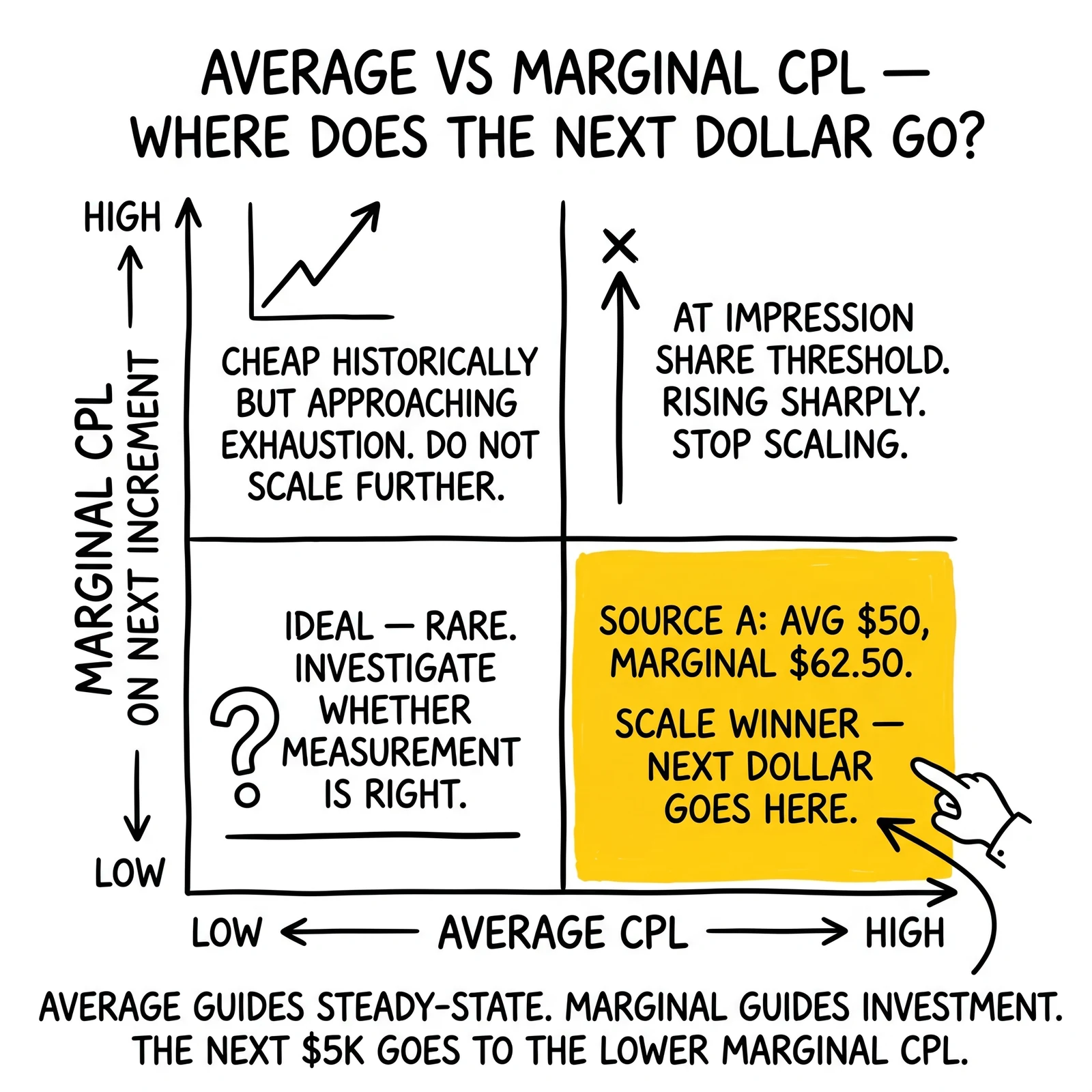
If Source A’s marginal CPL is $62.50 and Source B’s marginal CPL is $85, and both sources produce leads with similar net value, the next $5,000 goes to Source A. This remains true even if Source A has a higher average CPL than Source B – the marginal economics, not the average economics, determine where incremental spend produces more value.
Build a marginal CPL estimate for each source by analyzing the relationship between spend level and CPL across the past 6–12 months. Sources that have been held at static spend levels provide limited data for marginal cost estimation – deliberately vary spend levels in testing cycles to generate the data needed.
Return on Ad Spend vs. Return on Source Investment
ROAS as typically calculated is a platform metric: revenue attributed to a campaign divided by media spend. For source-level P&L, this metric is incomplete in two ways: it excludes non-media costs and it uses attribution logic that may misrepresent actual contribution.
Source-Level ROAS Calculation
For a more complete source-level ROAS:
Source ROAS = Net Revenue (Source) / Total Costs (Source, including overhead allocation)Using the Source A example from above:
- Net Revenue: $344,897
- Total Costs: Variable costs + Overhead = ($107,900 + $48,700) = $156,600
- Source ROAS: $344,897 / $156,600 = 2.20x
Compare to platform-reported ROAS for the same source, which typically divides gross revenue by media spend only: $374,400 / $104,000 = 3.60x.
The gap between 3.60x (platform-reported) and 2.20x (source P&L ROAS) represents the cost categories that platform dashboards exclude. For capital allocation decisions, the source P&L ROAS is the relevant number. The platform ROAS is useful for within-platform optimization (comparing ad sets, keywords, creatives) but should not drive cross-source investment decisions.
Attribution Adjustment for Source P&L
Source-level attribution is more straightforward than multi-touch attribution for full-funnel marketing because most lead generation sources are direct-response channels where the source generates the lead directly. The attribution question that complicates brand marketing – which touchpoint deserves credit for a consumer who saw six ads before converting – is less relevant for lead generation operations where most conversions happen within a single session from a specific source.
The attribution complexity that does matter in lead P&L is cross-source duplication: a consumer who submits through your Google Ads campaign and also through an affiliate channel. If both leads end up with the same buyer, one gets returned as a duplicate. The source that generated the returned lead should record that return in its P&L, which is why return attribution by source matters.
Building the Model: Practical Implementation
The source-level P&L model is most useful when it runs on a consistent cadence against clean data. The following implementation sequence builds toward a functional model without requiring an immediate rebuild of data infrastructure.
Phase 1: Revenue and Returns by Source (Month 1)
Before overhead allocation, establish clean revenue and return attribution by source. This requires:
- Lead records tagged with source ID at generation
- Return records tagged with originating lead source ID
- A monthly extract that aggregates gross revenue and returns by source
Most distribution platforms (boberdoo, LeadExec, LeadsPedia, Phonexa) support source-tagged reporting. The data extraction may require a custom report configuration or API pull rather than using default dashboards.
Output: A monthly spreadsheet with columns: Source | Gross Leads | Return Rate | Net Delivered | Gross Revenue | Return Deductions | Net Revenue
Phase 2: Variable Cost Attribution (Month 2)
Add variable costs to the monthly source report. Sources:
- Media cost by source: from ad platform exports or affiliate network reports
- Per-lead validation and certification fees: aggregate from vendor invoices divided by source lead volume, or per-lead if vendor systems support source-level cost reporting
- Distribution platform per-lead fees: from platform billing reports
Output: Extended spreadsheet adding columns: Media Cost | Per-Lead Tech Fees | Certification Costs | Variable Contribution | Variable Margin %
Phase 3: Overhead Allocation (Month 3)
Add overhead allocation using the methodologies above. This requires:
- Monthly overhead cost by category from accounting
- Allocation basis by category (volume proportion, revenue proportion, time allocation)
- Calculation of each source’s overhead allocation
Output: Complete source P&L with net contribution and net margin columns
Phase 4: Marginal Cost Estimation and Aging Analysis (Month 4+)
With three months of source-level data, build:
- Marginal CPL estimates by testing spend variation against lead output over time
- Aging cost by source by tracking sell-through rates and price by aging tier
- Float cost by source based on buyer payment term data
Output: Full source-level economics model including aging and float, marginal cost curves by source
Using the Model: Decision Triggers
The model is useful only insofar as it drives decisions. Common decision triggers from source-level P&L analysis:
Source termination: Net contribution below 15% for two consecutive months after remediation attempts. At this margin level, the source is consuming overhead capacity and management attention that generates more value applied to better-performing sources.
Source scale increase: Net contribution above 50% with marginal CPL below average CPL. Both conditions together confirm that additional spend at this source will generate above-average returns at below-average incremental cost.
Source renegotiation: Variable margin is strong (above 50%) but overhead allocation is disproportionately high due to buyer relationship management or compliance infrastructure. Renegotiate supplier terms or restructure the relationship to reduce overhead burden.
Aging cost remediation: Source produces acceptable variable margin but aging cost exceeds $5/lead, indicating high non-sale-through rates. Investigate why leads from this source are not selling at real-time prices – timing, geographic concentration, or qualification issues.
Float cost review: Source float cost exceeds $1/lead. Evaluate whether the buyers purchasing this source’s leads can be moved to faster payment terms, or whether the source should be repriced to reflect higher float burden.
Frequently Asked Questions
How often should I run the source-level P&L model?
Monthly minimum. Weekly for high-volume operations where source economics can shift quickly. The monthly cadence catches trends before they compound into structural problems. Quarterly review of marginal cost curves and aging analysis is sufficient given the slower-moving nature of those metrics.
My distribution platform does not tag returns with source IDs. How do I handle return attribution?
The manual workaround is maintaining a lookup table of lead IDs with their source tags, then joining return data to that table. This requires capturing lead IDs in your source tracking and retaining them for the duration of the return window plus buffer. Most distribution platforms store lead IDs that can be cross-referenced – the issue is typically extracting and joining the data, not availability.
How should I handle sources that feed multiple buyers with different payment terms?
Calculate a weighted average payment term for each source based on the distribution of volume across buyers with different payment terms. If 60% of Source A’s leads go to a buyer on net-15 and 40% go to buyers on net-45, the weighted average payment term is (0.6 × 15) + (0.4 × 45) = 27 days. Use this weighted average in the float cost calculation.
What is the right overhead allocation for a small operation with one or two team members?
For small operations, precise overhead allocation adds less value than understanding the rough magnitude. Estimate 20–25% of gross revenue as overhead for a one-to-two-person operation (covering platform subscriptions, legal, compliance, and implicit labor cost). This rough allocation identifies whether source variable margins cover overhead at all – the key question for small operations – without requiring detailed allocation methodology.
How do I calculate marginal CPL if I have never varied spend levels by source?
Run a controlled spend variation test over 30 days: increase spend by 20% on your largest source and measure the CPL impact. If CPL rises 5%, marginal CPL is approximately $50 × (1 + 0.05/0.20) = $62.50 at the margin (assuming linear relationship, which is an approximation). Repeat at the next level to build a more complete marginal cost curve.
At what lead volume does source-level P&L modeling become worth the investment?
The model pays for itself when the operation processes more than 2,000 leads monthly from three or more distinct sources. Below that threshold, the source-level variation is visible without formal modeling. Above 5,000 monthly leads from five or more sources, formal modeling is essential – the variation becomes too complex to manage without structured analysis.
Key Takeaways
Blended P&L hides the sources that are subsidizing each other. A source running negative net margin can survive indefinitely inside an operation with strong overall margins – until it cannot. Source-level visibility surfaces this before the problem becomes structural.
Return rate affects source economics at two levels. The gross revenue impact (refunds issued) and the processing cost impact (labor per return) both belong in the source P&L. Return rate metrics without processing cost attribution understate the true cost of high-return sources.
Aging cost is a structural penalty on certain sources. Sources generating traffic concentrated in low-demand windows or with weaker intent signals incur aging costs that never appear in average CPL metrics. Track sell-through rates by source to identify and quantify this margin compression.
Payment terms create a float burden that differs by source. Sources feeding buyers with slow payment cycles cost more to finance than sources feeding buyers with fast payment terms. Float cost allocation makes this visible in source contribution margins.
Marginal CPL, not average CPL, determines where the next dollar should go. Average cost analysis guides steady-state operations. Scaling decisions require marginal cost analysis. A source with higher average CPL but lower marginal CPL at the next increment deserves the next investment before a source with lower average CPL that is approaching inventory exhaustion.
Overhead allocation methodology matters less than consistency. Choose volume-proportional or revenue-proportional allocation for each overhead category, document the choice, and apply it consistently. Changing methodologies between periods makes trend analysis unreliable and undermines the model’s utility for tracking progress.
The model generates value through decisions, not through reports. A beautiful source P&L that does not trigger terminations, renegotiations, or reallocations is an accounting exercise, not a management tool. The standard for success is whether source-level analysis changes where capital is allocated.
Sources
- Phonexa Platform Documentation – Lead distribution platform with source-tagged routing, return tracking, and per-lead cost reporting capabilities
- LeadsPedia – Affiliate tracking and lead distribution platform with source-level revenue and disposition reporting
- boberdoo Lead Distribution – Lead management software with per-source P&L reporting and buyer integration tools
- ActiveProspect TrustedForm – Per-lead consent certification with source-attributable cost tracking
- Womble Bond Dickinson, “TCPA Litigation Survey” (2018) – Industry reference for TCPA settlement cost benchmarks used in compliance reserve calculations
Financial examples are illustrative. Actual source economics vary by vertical, buyer relationships, traffic quality, and operational scale. Validate model assumptions against your specific cost structure before using outputs for capital allocation decisions.